Data Brief Description:

The data in question come from a study that involved a one-week ecological momentary assessment (EMA) protocol. For seven consecutive days, participants (N=127) responded to 10 prompts delivered at pseudo-random times. The timing of EMA probes was built around class schedules during the day (hence pseudo-random). More detail about the sample and procedures can be found here.

Imputation Options

There are several imputation packages available that aid researchers imputing data in R. Perhaps the two most popular are the mice package (van Buuren and Groothuis-Oudshoorn 2011) and the Amelia package (Honaker, King, and Blackwell 2011). When the data in question has a nested structure (e.g., students nested within classrooms, patients nested within clinics, observations nested within individuals, etc.), the pan package (Zhao and Schafer 2018) can be used.

In this case, I will be using the mitml package (Grund, Robitzsch, and Luedtke 2018), which is a wraparound package that depends on the pan package. Alternative approaches using the pan algorithm via mice can be found here.

Imputation Model

To setup the imputation model, I need to specify the variables that need to be imputed (in front of the ~) and the complete variables, along with the random effects (after the ~). Exploratory analyses covered in the first post indicated that BFI Openess scores and BFI Conscientiousness scores both predicted missingness. As is common practice, I will also include dispositional negativity scores, which serve as the primary individual-level predictor in my final model.

fml<- c.Worst + c.Best + NegAff + PosAff  ~ 
  1 + c.DN + BFI_C + BFI_O + (1|ID)

With the formula setup, I can now impute the data. There have been a number of recommendations out there regarding how many datasets you need to impute to ensure that you get stable results. I recommend reading a pair of papers out there if you are convinced that you can always get away with using 10 datasets when imputing (Bodner 2008; Graham, Olchowski, and Gilreath 2007).

Based on the structure of my data and the total missingness and recommendations made by Graham, Olchowski, and Gilreath (2007), I chose to impute 20 data sets. I also have a relatively lengthy burn-in period so I can ensure convergence of the posterior distributions from which values are drawn. In setting n.iter = 50 I have further made the choice to separate my draws from the MCMC chains to help mitigate any autocorrelation that could arise in imputed data sets. These are all settings that can be played around with and using diagnostic plots along the way is the main tool for checking the imputation was successful and did not introduce its own artifacts into the analysis.

imp<-panImpute(dat.study1, 
               formula=fml, 
               n.burn=100, 
               n.iter = 50, 
               m=20, 
               seed = 0716)

Extracting Datasets

The next step is to pull out the imputed data and start examining whether or not the imputed data sets make sense. First, we can examine convergence of the imputation model. To give a concrete example of using diagnostic plots if you run plot(imp, print='beta') you would be able review convergence for the \(\beta\) parameters (the regression coefficients) in the model. Doing so would also reveal that some parameters did not fully converge and the number of iterations between draws likely needs to be increased. To address these problems, I begin by re-running the imputation model with a longer burn-in phase and greater distance between draws.

imp<-panImpute(dat.study1, 
               formula=fml, 
               n.burn=10000, 
               n.iter = 5000, 
               m=20, 
               seed = 0716)

Having satisfied myself that there are no lingering convergence issues I can create some initial plots. First, I need to re-structure the data to make it a bit easier to plot.

dat<-mitmlComplete(imp)

dat.long<-data.frame()
for(i in 1:20){
  dat.temp<-dat[[i]]
  dat.temp$IMP<-rep(i, length(dat.temp[,1]))
  dat.long<-rbind(dat.long, dat.temp)
}

dat.study1$IMP<-rep(0, length(dat.study1[,1]))
dat.long<-rbind(dat.study1, dat.long)
dat.long$Orig<-ifelse(dat.long$IMP<1, 'Original', 'Imputed')

Okay now we can plot the results.

g1<-ggplot()+
  geom_freqpoly(data = dat.long, aes(x=NegAff, group=IMP, color=Orig), stat = 'density')+
  theme(legend.title = element_blank())+
  ggtitle('Momentary Negative Affect')+
  ylab('Density')+
  xlab('')

g2<-ggplot()+
  geom_freqpoly(data = dat.long, aes(x=PosAff, group=IMP, color=Orig), stat = 'density')+
  theme(legend.title = element_blank())+
  ggtitle('Momentary Positive Affect')+
  ylab('Density')+
  xlab('')

g3<-ggplot()+
  geom_freqpoly(data = dat.long, aes(x=c.Worst, group=IMP, color=Orig), stat = 'density')+
  theme(legend.title = element_blank())+
  ggtitle('Worst Event')+
  ylab('Density')+
  xlab('')

g4<-ggplot()+
  geom_freqpoly(data = dat.long, aes(x=c.Best, group=IMP, color=Orig), stat = 'density')+
  theme(legend.title = element_blank())+
  ggtitle('Best Event')+
  ylab('Density')+
  xlab('')

print(cowplot::plot_grid(g1, g2, g3, g4))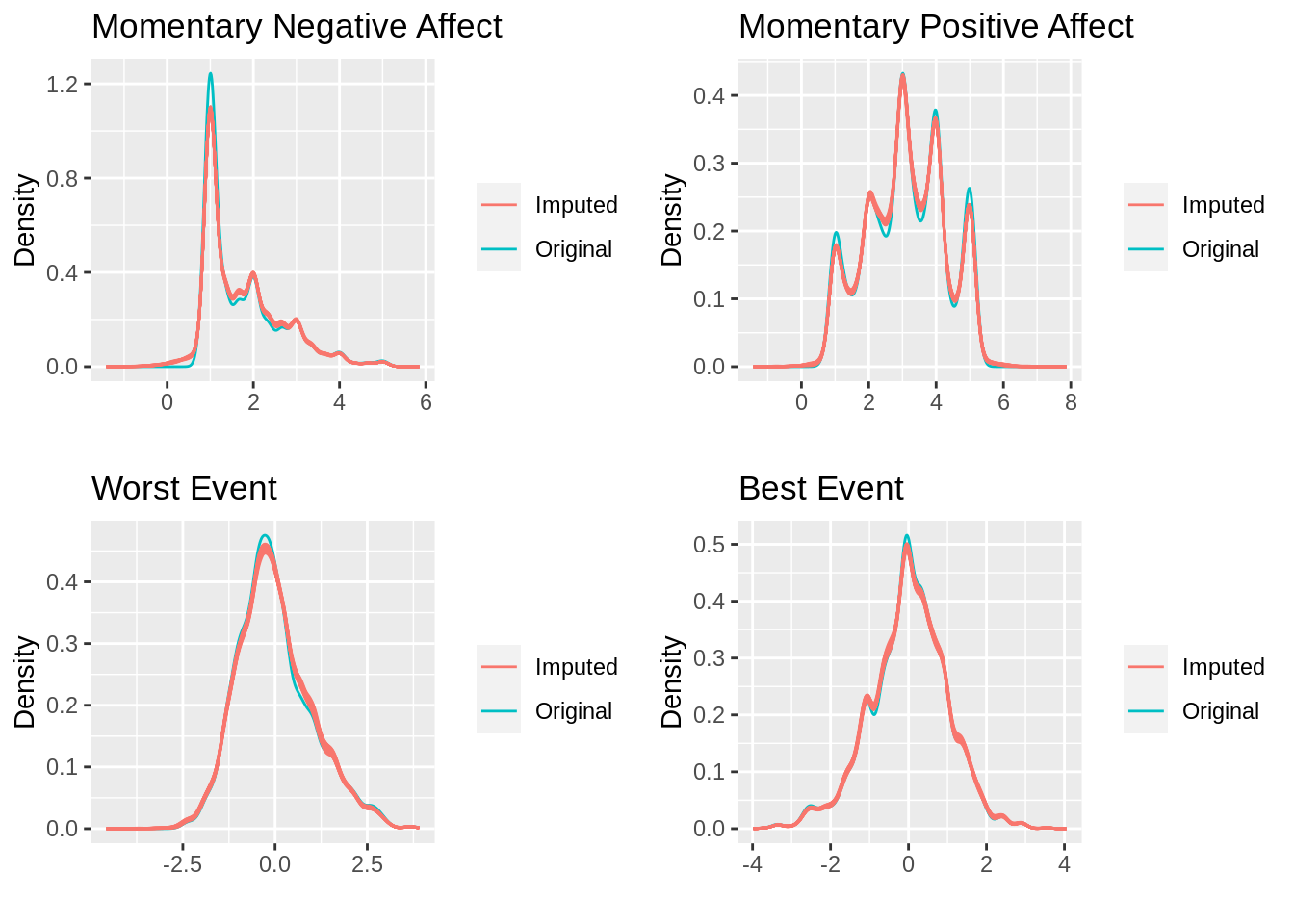

The good news is that the imputed values largely follow the same distribution as the original values. Having assessed convergence and now the actual imputation results, I feel pretty good about the results. I am now ready to move on to the actual analysis, which will be reviewed in the final post in this series.

References

Bodner, Todd E. 2008. “What improves with increased missing data imputations?” Structural Equation Modeling 15 (4): 651–75. https://doi.org/10.1080/10705510802339072.
Graham, John W., Allison E. Olchowski, and Tamika D. Gilreath. 2007. “How many imputations are really needed? Some practical clarifications of multiple imputation theory.” Prevention Science 8 (3): 206–13. https://doi.org/10.1007/s11121-007-0070-9.
Grund, Simon, Alexander Robitzsch, and Oliver Luedtke. 2018. Mitml: Tools for Multiple Imputation in Multilevel Modeling. https://CRAN.R-project.org/package=mitml.
Honaker, James, Gary King, and Matthew Blackwell. 2011. “Amelia II: A Program for Missing Data.” Journal of Statistical Software 45 (7): 1–47. http://www.jstatsoft.org/v45/i07/.
van Buuren, Stef, and Karin Groothuis-Oudshoorn. 2011. “mice: Multivariate Imputation by Chained Equations in R.” Journal of Statistical Software 45 (3): 1–67. https://www.jstatsoft.org/v45/i03/.
Zhao, Jing Hua, and Joseph L. Schafer. 2018. Pan: Multiple Imputation for Multivariate Panel or Clustered Data.