By Matthew Barstead, Ph.D. | July 11, 2018
Long ago (the first half of my grad school life), I created a model for a manuscript I submitted. The paper was focused on adolescents’ appraisals of their relationships with their mothers, fathers, and best friends. Specifically, I wanted to test whether the association between different motivations for social withdrawal (i.e., removing oneself from social activities and interactions) and internalizing symptoms varied as a function of perceived support in any one (or all three) of these relationships.
It is and was a modest study, with some flaws (notably the fact I only had self-report measures from the adolescents). If you want more context for the rest of this post, you can read the paper here. These data come from the Friendship Project and were collected in the early-to-mid 2000s, a fact that I wish I had included in the manuscript in retrospect. My blog is as good a place as any to call out my past transparency shortcomings I suppose.
To understand the data and models, here is some additional information:
- I had grade 8 measures of relationship quality, shyness, preference for solitude, and anxiety/depression
- I had grade 9 measures of anxiety and depression
- The analyses were based on a saturated path model in
lavaan- an R package for creating and testing structural equation models.
Using lavaan (latent variable analysis), I created three latent variables that represented outcomes of interest in grade 9: anxiety, depression, and general negative affect (I refer to this as dispositional negativity in the manuscript). To start, here is the model:
library(lavaan)
mod8<-'
int=~cdi9ngmd+cdi9inpr+cdi9inef+cdi9anhe+cdi9ngse+masc9tr+masc9sma+masc9per+masc9ac+masc9hr+masc9pf
dep=~cdi9ngmd+cdi9inpr+cdi9inef+cdi9anhe+cdi9ngse
anx=~masc9tr+masc9sma+masc9per+masc9ac+masc9hr+masc9pf
int~ysr8anxd+sex1+c.pfs+c.shy+
c.mospt+mopstXpfs+mopstXshy+
c.faspt+
c.frspt
dep~ysr8anxd+sex1+c.pfs+c.shy+
c.mospt+mopstXpfs+mopstXshy+
c.faspt+
c.frspt+frsptXpfs+frsptXshy
anx~ysr8anxd+sex1+c.pfs+c.shy+
c.mospt+mopstXpfs+mopstXshy+
c.faspt+
c.frspt
#Covariances
int~~0*dep
int~~0*anx
anx~~0*dep
#Added covariances
masc9hr ~~ masc9pf
cdi9inpr ~~ masc9per
cdi9inef ~~  masc9ac
'

fit8<-sem(mod8, data=dat, std.lv = T, estimator = 'MLR')
summary(fit8, fit.measures=T, standardized=T, rsquare=T)
## lavaan 0.6-5 ended normally after 66 iterations
##
## Estimator ML
## Optimization method NLMINB
## Number of free parameters 65
##
## Used Total
## Number of observations 188 330
##
## Model Test User Model:
## Standard Robust
## Test Statistic 226.515 221.684
## Degrees of freedom 122 122
## P-value (Chi-square) 0.000 0.000
## Scaling correction factor 1.022
## for the Yuan-Bentler correction (Mplus variant)
##
## Model Test Baseline Model:
##
## Test statistic 1392.959 1307.712
## Degrees of freedom 176 176
## P-value 0.000 0.000
## Scaling correction factor 1.065
##
## User Model versus Baseline Model:
##
## Comparative Fit Index (CFI) 0.914 0.912
## Tucker-Lewis Index (TLI) 0.876 0.873
##
## Robust Comparative Fit Index (CFI) 0.916
## Robust Tucker-Lewis Index (TLI) 0.878
##
## Loglikelihood and Information Criteria:
##
## Loglikelihood user model (H0) -3975.960 -3975.960
## Scaling correction factor 1.222
## for the MLR correction
## Loglikelihood unrestricted model (H1) -3862.702 -3862.702
## Scaling correction factor 1.091
## for the MLR correction
##
## Akaike (AIC) 8081.919 8081.919
## Bayesian (BIC) 8292.288 8292.288
## Sample-size adjusted Bayesian (BIC) 8086.402 8086.402
##
## Root Mean Square Error of Approximation:
##
## RMSEA 0.068 0.066
## 90 Percent confidence interval - lower 0.054 0.052
## 90 Percent confidence interval - upper 0.081 0.079
## P-value RMSEA <= 0.05 0.020 0.030
##
## Robust RMSEA 0.067
## 90 Percent confidence interval - lower 0.052
## 90 Percent confidence interval - upper 0.080
##
## Standardized Root Mean Square Residual:
##
## SRMR 0.049 0.049
##
## Parameter Estimates:
##
## Information Observed
## Observed information based on Hessian
## Standard errors Robust.huber.white
##
## Latent Variables:
## Estimate Std.Err z-value P(>|z|) Std.lv Std.all
## int =~
## cdi9ngmd 0.730 0.200 3.641 0.000 0.888 0.441
## cdi9inpr 0.203 0.088 2.318 0.020 0.247 0.290
## cdi9inef 0.490 0.166 2.944 0.003 0.597 0.380
## cdi9anhe 1.237 0.207 5.985 0.000 1.506 0.637
## cdi9ngse 0.577 0.134 4.308 0.000 0.702 0.470
## masc9tr 1.573 0.248 6.345 0.000 1.915 0.650
## masc9sma 1.447 0.218 6.645 0.000 1.761 0.679
## masc9per -0.733 0.299 -2.454 0.014 -0.892 -0.368
## masc9ac -0.644 0.373 -1.728 0.084 -0.784 -0.237
## masc9hr 1.117 0.309 3.616 0.000 1.360 0.386
## masc9pf 0.837 0.252 3.323 0.001 1.019 0.381
## dep =~
## cdi9ngmd 1.180 0.183 6.445 0.000 1.298 0.645
## cdi9inpr 0.396 0.064 6.151 0.000 0.436 0.511
## cdi9inef 0.789 0.146 5.402 0.000 0.868 0.553
## cdi9anhe 1.185 0.184 6.442 0.000 1.304 0.551
## cdi9ngse 0.971 0.141 6.876 0.000 1.068 0.714
## anx =~
## masc9tr 0.999 0.290 3.449 0.001 1.248 0.423
## masc9sma 0.749 0.245 3.052 0.002 0.935 0.361
## masc9per 1.381 0.241 5.730 0.000 1.725 0.711
## masc9ac 2.168 0.276 7.861 0.000 2.708 0.817
## masc9hr 1.296 0.262 4.955 0.000 1.618 0.459
## masc9pf 1.129 0.208 5.431 0.000 1.410 0.527
##
## Regressions:
## Estimate Std.Err z-value P(>|z|) Std.lv Std.all
## int ~
## ysr8anxd 0.121 0.042 2.919 0.004 0.100 0.368
## sex1 0.071 0.254 0.280 0.780 0.058 0.029
## c.pfs -0.097 0.163 -0.593 0.553 -0.080 -0.064
## c.shy 0.408 0.183 2.227 0.026 0.335 0.213
## c.mospt -0.337 0.186 -1.814 0.070 -0.277 -0.153
## mopstXpfs -0.219 0.211 -1.039 0.299 -0.180 -0.089
## mopstXshy -0.437 0.279 -1.568 0.117 -0.359 -0.128
## c.faspt 0.041 0.165 0.251 0.802 0.034 0.023
## c.frspt -0.176 0.210 -0.838 0.402 -0.145 -0.081
## dep ~
## ysr8anxd 0.037 0.039 0.952 0.341 0.034 0.126
## sex1 0.085 0.221 0.386 0.700 0.077 0.039
## c.pfs -0.039 0.136 -0.286 0.775 -0.035 -0.028
## c.shy -0.186 0.180 -1.035 0.301 -0.169 -0.107
## c.mospt -0.212 0.182 -1.168 0.243 -0.193 -0.107
## mopstXpfs 0.211 0.250 0.843 0.399 0.191 0.094
## mopstXshy -0.178 0.255 -0.698 0.485 -0.162 -0.058
## c.faspt -0.219 0.124 -1.768 0.077 -0.199 -0.137
## c.frspt 0.029 0.193 0.148 0.883 0.026 0.014
## frsptXpfs -0.414 0.213 -1.944 0.052 -0.377 -0.257
## frsptXshy 0.847 0.268 3.159 0.002 0.770 0.282
## anx ~
## ysr8anxd 0.122 0.034 3.562 0.000 0.098 0.362
## sex1 0.391 0.220 1.780 0.075 0.313 0.156
## c.pfs 0.321 0.137 2.348 0.019 0.257 0.207
## c.shy 0.411 0.188 2.187 0.029 0.329 0.209
## c.mospt 0.172 0.191 0.901 0.368 0.138 0.076
## mopstXpfs 0.110 0.217 0.508 0.612 0.088 0.043
## mopstXshy -0.112 0.269 -0.418 0.676 -0.090 -0.032
## c.faspt 0.102 0.142 0.716 0.474 0.082 0.056
## c.frspt 0.108 0.191 0.567 0.570 0.087 0.048
##
## Covariances:
## Estimate Std.Err z-value P(>|z|) Std.lv Std.all
## .int ~~
## .dep 0.000 0.000 0.000
## .anx 0.000 0.000 0.000
## .dep ~~
## .anx 0.000 0.000 0.000
## .masc9hr ~~
## .masc9pf 1.917 0.512 3.746 0.000 1.917 0.392
## .cdi9inpr ~~
## .masc9per -0.351 0.129 -2.723 0.006 -0.351 -0.305
## .cdi9inef ~~
## .masc9ac -0.311 0.219 -1.417 0.156 -0.311 -0.135
##
## Variances:
## Estimate Std.Err z-value P(>|z|) Std.lv Std.all
## .cdi9ngmd 1.493 0.270 5.524 0.000 1.493 0.369
## .cdi9inpr 0.469 0.097 4.822 0.000 0.469 0.644
## .cdi9inef 1.320 0.187 7.075 0.000 1.320 0.535
## .cdi9anhe 1.483 0.265 5.592 0.000 1.483 0.265
## .cdi9ngse 0.547 0.123 4.450 0.000 0.547 0.245
## .masc9tr 2.346 0.392 5.985 0.000 2.346 0.270
## .masc9sma 1.977 0.373 5.293 0.000 1.977 0.294
## .masc9per 2.831 0.714 3.965 0.000 2.831 0.481
## .masc9ac 4.023 1.250 3.217 0.001 4.023 0.367
## .masc9hr 6.933 0.895 7.747 0.000 6.933 0.558
## .masc9pf 3.458 0.471 7.345 0.000 3.458 0.483
## .int 1.000 0.675 0.675
## .dep 1.000 0.826 0.826
## .anx 1.000 0.641 0.641
##
## R-Square:
## Estimate
## cdi9ngmd 0.631
## cdi9inpr 0.356
## cdi9inef 0.465
## cdi9anhe 0.735
## cdi9ngse 0.755
## masc9tr 0.730
## masc9sma 0.706
## masc9per 0.519
## masc9ac 0.633
## masc9hr 0.442
## masc9pf 0.517
## int 0.325
## dep 0.174
## anx 0.359Now there is a whole script file of assumption checking and model evaluation that goes along with this (that is how I got to model 8). I have just included the final model here for simplicity’s sake.
One thing that frustrates me when we report on interactions between variables is that we often pick static, potentially arbitrary values to probe simple slopes. A common pair of values is +/- 1 SD. Sometimes researchers will also examine simple slopes at the mean of the sample as well. Probing simple slopes at static values also influences how researchers present their findings visually. Typically, we get either a pair of bars or lines to use to help us better evaluate the nature of the detected interaction.
Here is where my gripe starts to eek in. Why are we probing simple slopes at static (often arbitrary) values? When our moderators are continuous? It seems to me the better approach is to evaluate and interpret the effect of the moderator on the association between X and Y along the entire continuum of plausible moderator values.
To do this, I need to extract some information from my model first. I’ll need the point estimates and their variances invovled in defining the moderation (pro-tip, I am using the parm[,1:3] line to figure out the correct numbering for the parameters in the model):
parm<-as.data.frame(parameterEstimates(fit8))
parm[,1:3]

COV<-vcov(fit8)
COVd<-as.data.frame(COV)
Okay so now that I have the information, I can grab the relevant values as follows. (You don’t need to grab things from the model using R objects - you can type in values manually here instead should you wish).
b1<-parm[26,4]#slope for SHY
b3<-parm[29,4]#slope for SHY x Maternal Support
s11<-COV[26,26]#variance for SHY
s13<-COV[26,29]#covariance for SHY and SHY x Maternal Support
s33<-COV[29,29]#variance for SHY x MS Parameter
I then need to create a vector of values that I am going to use for plotting. Since the long-standing convention has been to use standardized values of the moderator for probing simple slopes, I keep with that tradition in the code below.
sd1<-c(-2, -1.75, -1.5, -1.25, -1, -.75, -.5, -.25, 0,
       .25,.5,.75,1,1.25,1.5,1.75,2)

sd2<-sd1*sd(dat$c.mospt)

#Formula for standard error of simple slopes can be found in most regression textbooks
se<-sqrt(s11+2*(sd2)*s13+(sd2)*(sd2)*s33)
se
## [1] 0.3605632 0.3259049 0.2928709 0.2620761 0.2344049 0.2110890 0.1937077
## [8] 0.1839510 0.1830423 0.1911077 0.2071014 0.2293710 0.2562856 0.2865392
## [15] 0.3191838 0.3535578 0.3892032b1<-b1+b3*(sd2)
b1## [1] 1.94764891 1.75514194 1.56263497 1.37012800 1.17762103 0.98511406
## [7] 0.79260710 0.60010013 0.40759316 0.21508619 0.02257922 -0.16992775
## [13] -0.36243472 -0.55494169 -0.74744865 -0.93995562 -1.13246259UB<-b1+se*qnorm(.975)
LB<-b1+se*qnorm(.025)
DF.temp<-data.frame(b1, sd1, UB, LB)
library(ggplot2)
g1<-ggplot(DF.temp)+
geom_ribbon(aes(ymin=LB, ymax=UB, x=sd1), alpha=.7)+
geom_line(aes(y=b1, x=sd1))+
geom_hline(aes(yintercept=0), lty='dashed')+
xlab('Standardized Maternal Support Scores')+
ylab('Simple Slope for Shyness-DN Association')+
ggtitle("Shyness Predicting Dispositional Negativity as a Function of Maternal Support")
g1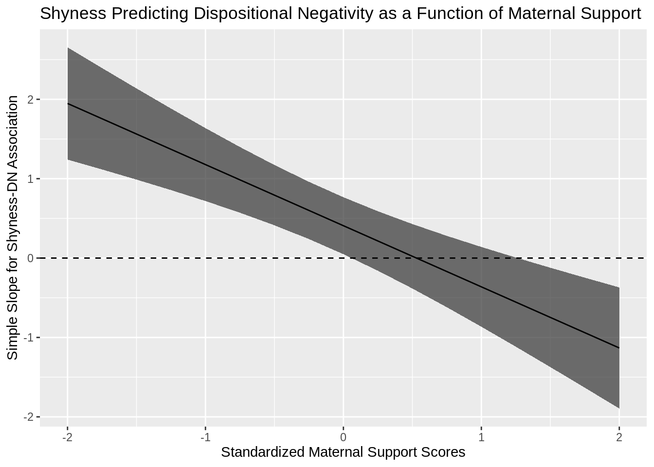
And voila! To me, the greatest value of this approach is that I can see exactly where 0 is included in the 95% confidence band and where the value falls outside the confidence band. For instance, in the plot above, I can easily see that the model would only predict a significant and positive association between shyness and dispositional negativity for adolescents with lower levels of self-reported maternal relationship quality.
Note that you may have to change the y-axis scaling to get the plot to display correctly. Otherwise, you now never have to ever ever plot the interaction between two continuous variables using a pair of static variables.