Data Brief Description:

The data in question come from a study that involved a one-week ecological momentary assessment (EMA) protocol. For seven consecutive days, participants (N=127) responded to 10 prompts delivered at pseudo-random times. The timing of EMA probes was built around class schedules during the day (hence pseudo-random). More detail about the sample and procedures can be found here.

As might be expected, some prompts were not responded to or were responded to outside the response time window (which was 30 minutes in this case). In the present data set, what I cared about was predicting momentary mood using a measure of trait negativity (sometimes referred to as neuroticism, negative emotionality, or dispositional negativity).

The problem is that I believe that there are certain factors about individuals that make them less likely to complete all of their surveys. Technically speaking, I believe that the data are likely missing at random (that is that missingness is conditional on some set of predictors/covariates but not on the outcome measure).

There is a debate over whether researchers should impute or simply use full information maximum likelihood to address missingness in cases like the one represented by this current set of data. All things being equal, properly specified models using either approach will result in essentially the same result. Full information maximum likelihood (FIML) estimation is convenient, when it can be used, as it is often seamlessly intergrated into the modeling sofware.

The seamlessness of its integration can, however, sometimes lead to bad modeling practices. Being a little out of sight and a little out of mind, relying on FIML to resolve the effects of missing data on biasing estimates can be just a hair too easy. On the user side it is: set up the model, click run, and wait, filled with the confidence that comes from being repeatedly told that FIML can be used to deal with missing data, often forgetting the caveat that this is only true so long as the technical condition of missingness at random is met.

When imputing, probing for predictors of missingness is built into the process. It is a step that cannot be skipped as you are essentially building a model with other variables in your data set to predict missing scores. For my money, imputation forces you to be more thoughtful in dealing with missingness. With FIML, it can be a little too easy to perform an analysis with little to no examination of the reasons for missingness.

Step 1 - Understanding and Exploring Missingness

Before anything else we need to understand a little about the missingness in the data. For starters, how much missingness are we talking about here? That is relatively simple to answer. But even before that, a few pieces of information that may help readers understand this data set a bit better in the form of some variable names and definitions:

ID: ID variable

EMA Variables
c.Worst: Individually mean-centered ratings of how unpleasant the worst event was that occurred in the past hour

c.Best: Individually mean-centered ratings of how pleasant the best event was that occurred in the past hour

NegAff: Three-item composite (scores can range from 1 to 5) assessing momentary negative affect - mostly anxious affect (i.e., anxious, worried, nervous)

PosAff: Three-item composite (scores can range from 1 to 5) assessing momentary positive affect - mostly cheerful affect (i.e., cheerful, happy, joyful)

Individual Variables:
c.DN: Mean-centered dispositional negativity scores (combination of Neuroticism from Big Five and additional items that tap the anxious facet of neuroticism)

BFI_O: Big Five Openness Factor

BFI_C: Big Five Conscientiousness Factor

BFI_E: Big Five Extraversion Factor

Dep: IDAS general depression score

Miscellaneous:
IMP: 0 is used to mark these data as “original” (will be useful after imputation)

miss: 1 if missing EMA measures, 0 if not (more on this later)

In this study design, missingness is possible in any one of the EMA variables, though in practice if one of the four scores in question were missing, all scores for that period were typically missing (only 2 instances when this was not the case - see figure below). To understand missingness in this data set a little better, let’s take a closer look, now that we have a better understanding of what every variable represents.

mice::md.pattern(dat.study1)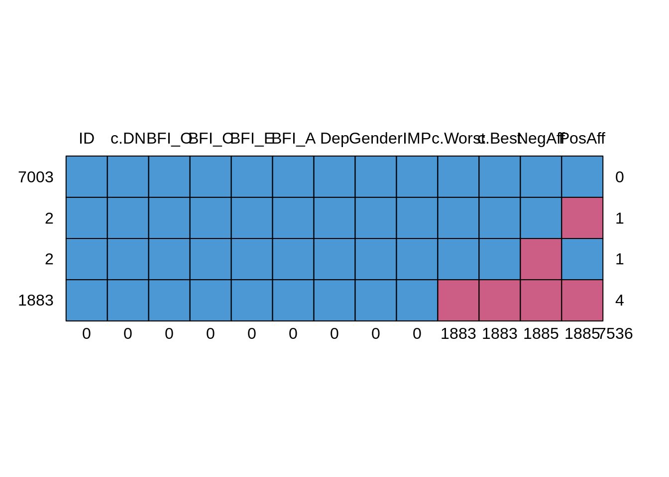

##      ID c.DN BFI_O BFI_C BFI_E BFI_A Dep Gender IMP c.Worst c.Best NegAff
## 7003  1    1     1     1     1     1   1      1   1       1      1      1
## 2     1    1     1     1     1     1   1      1   1       1      1      1
## 2     1    1     1     1     1     1   1      1   1       1      1      0
## 1883  1    1     1     1     1     1   1      1   1       0      0      0
##       0    0     0     0     0     0   0      0   0    1883   1883   1885
##      PosAff     
## 7003      1    0
## 2         0    1
## 2         1    1
## 1883      0    4
##        1885 7536

An alternative way to look at these data is to use the VIM package in R

VIM::aggr(
  dat.study1[
    c(
      'c.Worst', 
      'c.Best',
      'NegAff',
      'PosAff'
      )
    ]
  )

So now I can see that I am missing about 20% of data related to momentary events and mood. The next question is whether any of the individual-level variables available to me are related to missingness. First, I am going to need a indicator of missingness.

Let’s begin by getting a missingness variable in a new missing data set. Grabbing just the comlumns that I need from the original:

dat.miss<-data.frame(
  dat.study1[,c(1,4,7:12)], 
  miss = ifelse(!is.na(dat.study1$PosAff), "Complete", "Missing")
)

table(dat.miss$miss)

## 
## Complete  Missing 
##     7005     1885

With a proportion of .212 (i.e., \(\frac{1885}{8890} = .212\)), it looks as if I have successfully created my missingness variable. Now, it is time to plot. Let`s start with the 4 BFI factors.

g1<-ggplot(
  data = dat.miss, 
  aes(x=BFI_O, group=miss, color=miss)
  )+
  geom_freqpoly(stat = 'density')+
  theme(legend.title = element_blank())+
  ylab('')+
  xlab('BFI Openess Scores (1-5)')

g2<-ggplot(
  data = dat.miss, 
  aes(x=BFI_C, group=miss, color=miss)
  )+
  geom_freqpoly(stat = 'density')+
  theme(legend.title = element_blank())+
  ylab('')+
  xlab('BFI Conscientiousness Scores (1-5)')

g3<-ggplot(
  data = dat.miss, 
  aes(x=BFI_E, group=miss, color=miss)
  )+
  geom_freqpoly(stat = 'density')+
  theme(legend.title = element_blank())+
  ylab('')+
  xlab('BFI Extraversion Scores (1-5)')


g4<-ggplot(
  data = dat.miss, 
  aes(x=BFI_A, group=miss, color=miss)
  )+
  geom_freqpoly(stat = 'density')+
  theme(legend.title = element_blank())+
  ylab('')+
  xlab('BFI Agreeableness Scores (1-5)')

gridExtra::grid.arrange(g1, g2, g3, g4,
                        nrow=2)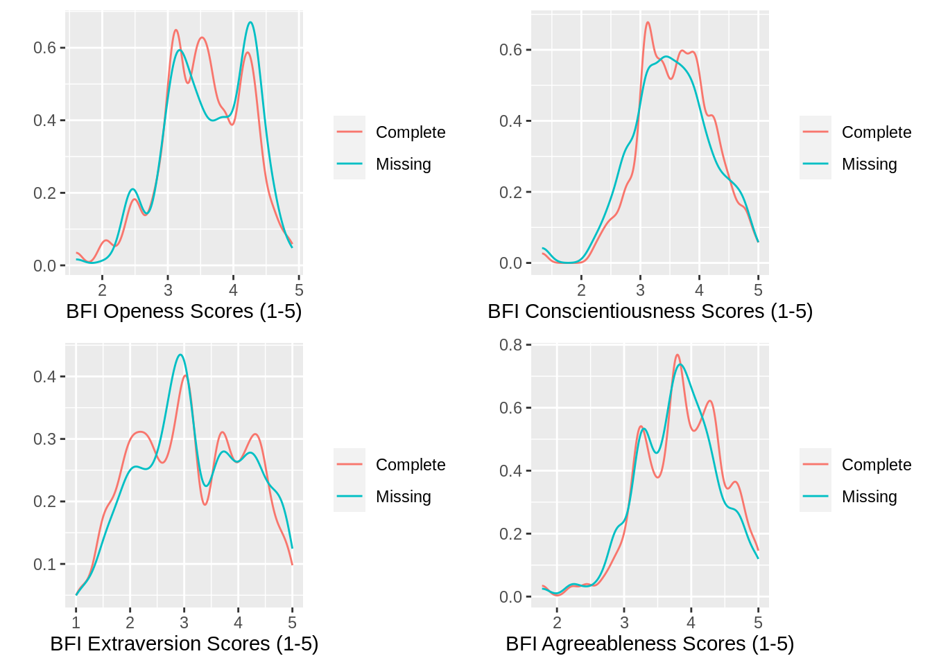

There is not much here that would suggest that missingness was related to these personality scores. The distributions look pretty similar. This is an empirical question, though and it is possible, therefore, to determine if any of these measures predict the likelihood of missingness. I am also not considering the nested nature of the data here, just plotting in an absolute sense. To address the issue on more empirical grounds then, I can use the lmer package.

fit.miss<-glmer(
  miss~1+BFI_O+BFI_C+BFI_E+BFI_A+(1|ID), 
  data=dat.miss, 
  family = 'binomial'
  )

fit.boot<-bootMer(fit.miss, 
                  FUN = fixef, 
                  nsim=5000, 
                  parallel='multicore', 
                  ncpus = 10
                  )

confint(fit.boot, type='perc')

## Bootstrap percent confidence intervals
## 
##                   2.5 %      97.5 %
## (Intercept) -1.94877015  0.19115816
## BFI_O        0.01754566  0.37859218
## BFI_C       -0.39542260 -0.01822857
## BFI_E       -0.05313720  0.18344948
## BFI_A       -0.37821070  0.01239628

According to this model, it seems as though the BFI Openness factor and the BFI Conscientiousness factor both predict the likelihood of failing to complete an assessment (i.e., 0 not included in the interval).

Let’s also look at our measures of dispositional negativity and general depression scores as potential variables of interest for the imputation model.

g5<-ggplot(
  data = dat.miss, 
  aes(x=c.DN, group=miss, color=miss)
  )+
  geom_freqpoly(stat = 'density')+
  theme(legend.title = element_blank())+
  ylab('')+
  xlab('Centered DN Scores')

g6<-ggplot(
  data = dat.miss, 
  aes(x=Dep, group=miss, color=miss)
  )+
  geom_freqpoly(stat = 'density')+
  theme(legend.title = element_blank())+
  ylab('')+
  xlab('IDAS Depression Scores')

gridExtra::grid.arrange(g5, g6,
                        nrow=1)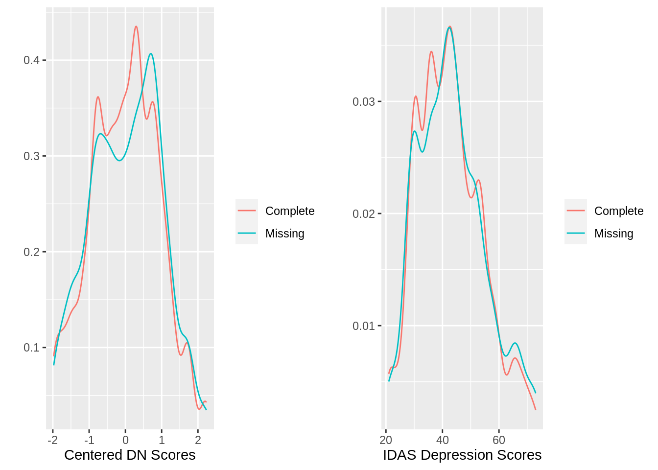

There is a little bit of a right shift in the distribution of DN scores when split by missing vs. complete. Since the two variables (depression and dispostional negativity scores) are also pretty strongly correlated (introducing a good deal of multicollinearity in the model), I am just going to use the dispositional negativity variable as it is most similar to the other personality variables examined above (also it is going in my model anyway). I also want to check to make sure that gender is not a factor in completion rates.

fit.miss2<-glmer(
  miss~1+c.DN+Gender+(1|ID), 
  data=dat.miss, 
  family = 'binomial', 
  )

fit.boot2<-bootMer(fit.miss2, 
                   FUN = fixef, 
                   nsim=5000, 
                   parallel='multicore', 
                   ncpus = 10
                   )

confint(fit.boot2, type = 'perc')

## Bootstrap percent confidence intervals
## 
##                  2.5 %      97.5 %
## (Intercept) -1.5177761 -1.16884330
## c.DN        -0.1188116  0.14345555
## Gender      -0.4123946  0.08398782

That is a no to DN and a no to Gender. At this stage, assuming these are the only relevant variables I have access to (in actuality there are more to consider in the complete data set - this is just a toy problem), I have identified the variables I will need to include when creating my imputation model.

Summary

Okay to wrap it up for post 1 of 3… Missing data is a problem when analyzing data sets, even relatively large ones. We know from decades of research that missingness can bias both estimates and their standard errors (depending on the reasons for missingness). Two techniques, FIML and multiple imputation have been used over the years to address the problems caused by missing data, when the technical condition of “missing at random” is met.

FIML is great and wonderful, but it can lead to bad practices owing to its ease of use (and often seamless integration with certain software tools). Multiple imputation can take longer and is a more invovled technique, but it forces you to think about the missingness more directly. An additional benefit is that multiple imputation will work with generally any type of statistical model, FIML by comparison requires maximum likelihood - an estimation that works for many but not all models.