By Matthew Barstead, Ph.D. | December 3, 2018
In the first post in this series, I described the impetus for this trek through statistical modeling, machine learning and artificial intelligence. I also provided an initial set of comparisons for three different approaches to classification: k-means, k-nearest neighbor, and latent profile analysis (model-based clustering). If you want to check those mini-walkthroughs out click here.
As a reminder, my goal here is to compare and contrast different approaches to data analysis and predictive modeling that are, in my mind, arbitrarily lumped into statistical modeling and machine learing/artificial intelligence categories. Though there may be some good reasons for dichotomizing statistics and machine learning, it has been my experience that each camp that favors one conceptualization over the other (i.e., statisticians vs. data scientists) holds unnecessary comtempt for the other group. On my shelf are textbooks that refer to linear regression models as supervised machine learning techniques (e.g., Zumel and Mount 2014) and statistical models (e.g., Gelman and Hill 2007). I promise that the ordinary least squares solution, regardless of how you categorize the technique, is going to return the same result given the same model and same data each time.
To remain consistent with the first post in this series, I am going to continue with the iris data set for now. The data set contains four measurements of plant anatomy: petal length, petal width, sepal length, and sepal width. These measures were collected on 50 specimens from three species for a total of 150 observations. The goal will be the same, continue to assess the accuracy of different classification techniques in predicting class membership using these data.
As opposed to the first post, each of the techniques I will employ in this post allow for classification of new data that a trained model has yet to “see.” The ability to predict out-of-sample data allows for a more applied series of testing scenarios. Specifically, I’ll evaluate each technique/model in terms of prediction accuracy using a k-fold cross validation technique.
The models covered in this post will include: naive Bayes classification, discriminant analysis, and multinomial logistic regression. The goal of each model is essentially the same - develop a model (or a series of mathematical rules if you prefer) that maximally predicts observed data and can be used to predict out of sample data (i.e., generalize to a population if you prefer).
Naive Bayes
Bayesian models have at their root a simple mathematical truism about the behavior of the probability of independent events. Bayes Theorem elegantly lays this truism out:
\[P(A|B) = \frac{P(B|A)P(A)}{P(B)}\]
The probability of \(A\) given the value of \(B\) is equal to the probability of \(B\) given \(A\) multiplied by the probability of \(A\) divided by the probability of \(B\). For those of you who know your way around a cross-tabulated table, these statements may seem pretty obvious. Let’s use some made up data to make it clearer though. Let’s model cancer risk as a function of smoking. I’ll pretend I was able to randomly sample 500 individuals from a population in which smokers are approximately 4 times more likely to receive a cancer diagnosis during their lifetime than non-smokers (Note I am just making these data up; I have no idea what appropriate base-rates should be). I am going to assume \(P(C|S)=.48\) (that is the probability of cancer given smoking) and \(P(C|NS)=.19\) (that is the probability of cancer given not-smoking).
P_C_sm<-.48
P_NC_sm<-1-P_C_sm
odds_C_sm<-P_C_sm/P_NC_sm

P_C_nsm<-.19
P_NC_nsm<-1-P_C_nsm
odds_C_nsm<-P_C_nsm/P_NC_nsm

odds_C_sm/odds_C_nsm
## [1] 3.935223An odds ratio of 3.94 would seem to confirm the fictional probabilities result in the scenario I outlined (i.e., smokers are 4x as likely to receive a cancer diagnosis). Now it is time to generate a random sample of each subpopulation. Let’s assume that smoking rates are relatively low in this population, say 15%. Since I am randomly sampling, I would expect that my final sample yields something close to this rate.
set.seed(143)
Smoker<-sample(c('Smoker', 'Non-Smoker'),
               prob=c(.15, .85),
               size=500,
               replace = TRUE)

Cancer<-vector()
for(i in 1:length(Smoker)){
  if(Smoker[i]=='Smoker'){
    Cancer[i]<-sample(c('Cancer', 'No Cancer'),
                      prob = c(P_C_sm, P_NC_sm),
                      size = 1)
  }
  else{
    Cancer[i]<-sample(c('Cancer', 'No Cancer'),
                      prob = c(P_C_nsm, P_NC_nsm),
                      size = 1)
  }
}

DF<-data.frame(Smoker=Smoker,
               Cancer=Cancer)
table(DF)
## Cancer
## Smoker Cancer No Cancer
## Non-Smoker 80 343
## Smoker 33 44So I now have a simple data set and I can, using Bayes Theorem calculating a probability of having cancer given the fact that an individual is a smoker \(P(C|S)\). We’ll just need some numbers to plug in. First some easy values, \(P(C)\) and \(P(S)\).
\[P(S) = \frac{33+44}{500} = .154\] \[P(C) = \frac{80+33}{500} = .226\]
Now, we need to get the probability of smoking, given cancer or \(P(S|C)\), which is just the same as saying, what is the probability of being a smoker, solely among individuals with cancer.
\[P(S|C) = \frac{33}{80+33}=.292\]
So now plugging this information into Bayes Theorem we get
\[P(C|S) = \frac{P(S|C)P(C)}{P(S)} = \frac{.292*.226}{.154}=.429\]
So there we have the probability of cancer given smoking is .429. What would we get if we looked at the probability of cancer given non-smoking status? We’ll need the value for \(P(NS|C)\), which is \(1-P(S|C)\) or \(.708\). We also need \(P(NS)\), which is \(1-P(S)\) or \(.846\).
\[P(C|NS) = \frac{P(NS|C)P(C)}{P(NS)} = \frac{.708*.226}{.846}=.189\]
This is the basic machinery of all Bayesian models, the naive Bayes classifier included. In this ficitious example we can see that smoking is associated with a more the 2-fold increase in the risk of a cancer diagnosis. Ideally, we would leverage this fact and other variables if we wanted to predict cancer risk.
One model that would enable the inclusion of additional variables is a Naive Bayes classifier. This model can handle mutinomial outcome variables (i.e., multiple categories) and continuous predictors or categorical predictors. The continuous predictors work best when approximately normal in their distribution as the probabilities used in the model are derived from the probability density function of the normal distrbution. These models calculate the conditional probability that a given case “belongs to” a particular category.
To compare the performance of the Naive Bayes classifier in accurately predicting out-of-sample cases, I’ll be using a k-fold cross validation technique in which I will hold out a randomly selected 20% of the cases from the iris data set as a testing sample, train the model on the remaining 80% and aggregate the prediction accuracy across on the testing and training set on 100 trials. With a small data set, this is a more effective technique to evaluate and compare model prediction performance than a single test/train split that could easily over- or underestimate out-of-sample prediction accuracy due to random chance.
data("iris")
set.seed(321)
k.fold<-100
library(e1071)

#Setting up a series of vectors for tracking accuracy
Start<-Sys.time()
Accuracy<-vector()
Model<-vector()
Pred_type<-vector()
for(i in 1:k.fold){
  #Split data into training/testing set
  smpl_size<-floor(.8*nrow(iris))
  ind <- sample(seq_len(nrow(iris)), size = smpl_size)
  train<-iris[ind, ]
  test<-iris[-ind, ]

  #Train the model and obtain accuracy based on observed data
  NB_train<-naiveBayes(Species~., data=train)
  NB_train_pred<-predict(NB_train, newdata = train)
  tab_train<-table(NB_train_pred, train$Species)
  Train_acc<-sum(diag(tab_train))/nrow(train)
  Accuracy<-c(Accuracy, Train_acc)
  Model<-c(Model, 'Naive Bayes')
  Pred_type<-c(Pred_type, 'Training Set')

  #Test model and get out of sample accuracy
  NB_test_pred<-predict(NB_train, newdata = test)
  tab_test<-table(NB_test_pred, test$Species)
  Test_acc<-sum(diag(tab_test))/nrow(test)
  Accuracy<-c(Accuracy, Test_acc)
  Model<-c(Model, 'Naive Bayes')
  Pred_type<-c(Pred_type, 'Testing Set')
}
round(Sys.time()-Start, digits = 2)
## Time difference of 1.53 secsSo not too long of a wait time to run through the cross-validation at 100 folds on my personal laptop.
Now, for the overall results of the model in terms of accurate predictions. I always prefer to show, my data whenever possible.
NB_KFold<-data.frame(Accuracy = Accuracy,
                     Model = Model,
                     Pred_type = Pred_type)

g1<-ggplot(data=NB_KFold, aes(x=Pred_type, y=Accuracy))+
  geom_bar(aes(fill=Pred_type),
           alpha=.5,
           stat='summary',
           fun.y='mean')+
  geom_point(aes(color=Pred_type),
             position = position_jitter(w = 0.05, h = 0))+
  coord_cartesian(ylim=c(.70, 1))+
  guides(fill=guide_legend(title=""),
         color=guide_legend(title = ""))+
  annotate(geom='text', x = 1, y = .75,
           label = paste('Mean =',
                         round(mean(NB_KFold$Accuracy[Pred_type=='Testing Set']),
                                         digits = 4)))+
  annotate(geom='text', x = 2, y = .75,
           label = paste('Mean =',
                         round(mean(NB_KFold$Accuracy[Pred_type=='Training Set']),
                                         digits = 4)))+
  theme_bw()
## Warning: Ignoring unknown parameters: fun.yg1## No summary function supplied, defaulting to `mean_se()`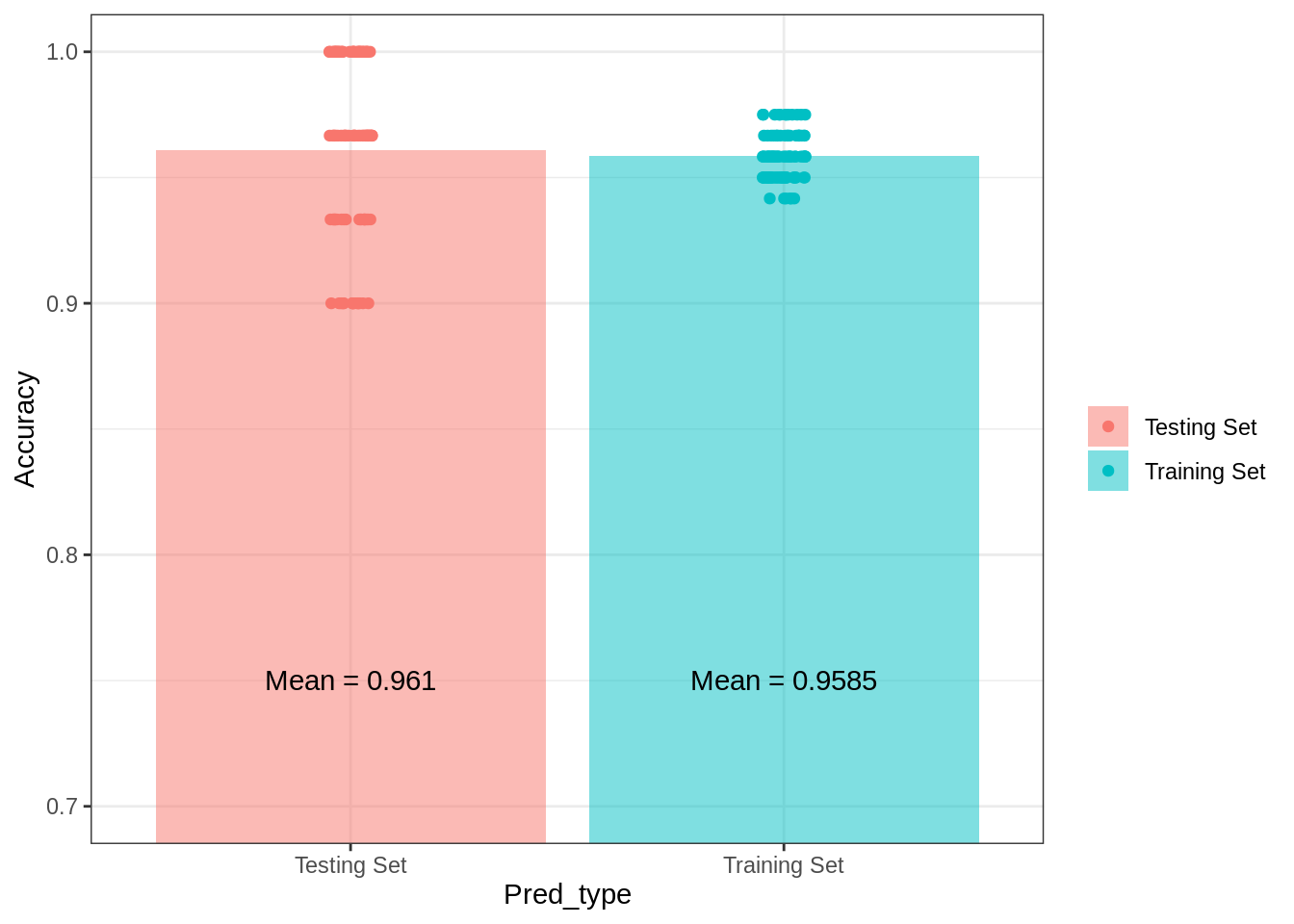
As expected, there is a slight dropoff in the accuracy of the model predictions when tested against out-of-sample data, but it really is slight. Prediction accuracy does show considerable range across the testing sets, however. Had I randomly selected one of the testing data sets that performs just above 80%, I would have likely come to a very different conclusion about the effectivenes of the model in predicting “unobserved” data. The point is that when evaluating model effectiveness it is important to keep in mind overall accuracy and the amount of variability in testing set accuracy..
For completeness and to allow a more direct comparison with the techniques described in the previous post in this series, below are the prediction results and confusion matrix for the entire iris sample using a Naive Bayes classifier.
NB_full<-naiveBayes(Species~., data = iris)
NB_full_pred<-predict(NB_full, newdata=iris)
table(NB_full_pred, iris$Species)
##
## NB_full_pred setosa versicolor virginica
## setosa 50 0 0
## versicolor 0 47 3
## virginica 0 3 47Note the number of errors presented in the confusion matrix above is still higher than the classification model presented at the end of the previous post (6 misclassified versus only 3).
Linear Discriminant Analysis
For individuals familiar with support vector machines, a linear discriminant analysis can be thought of as a special restrictive case of SVMs. Using a combination of linear functions, the model attempts to maximally separate the observed data into its constituent classifications or groupings. The discriminant function or functions represent linear combinations of the predictor variables, and as such have some similarities to principal components analyses as well. However, linear discriminant analyses are trying to categorize cases into groups, whereas principal components analyses are attempting to form clusters of variables.
Implementing a discriminant analysis is fairly straightforward. Borrowing from the code above, I’ll use the same cross-validation technique to assess model prediction performance.
data("iris")
set.seed(321)
k.fold<-100
library(MASS)

#Setting up a series of vectors for tracking accuracy
Start<-Sys.time()
Accuracy<-vector()
Model<-vector()
Pred_type<-vector()
for(i in 1:k.fold){
  #Split data into training/testing set
  smpl_size<-floor(.8*nrow(iris))
  ind <- sample(seq_len(nrow(iris)), size = smpl_size)
  train<-iris[ind, ]
  test<-iris[-ind, ]

  #Train the model and obtain accuracy based on observed data
  LDA_train<-lda(Species~., data=train)
  #note the inclusion of $class here - the way an lda object is stored
  LDA_train_pred<-predict(LDA_train, newdata = train)$class
  tab_train<-table(LDA_train_pred, train$Species)
  Train_acc<-sum(diag(tab_train))/nrow(train)
  Accuracy<-c(Accuracy, Train_acc)
  Model<-c(Model, 'LDA')
  Pred_type<-c(Pred_type, 'Training Set')

  #Test model and get out of sample accuracy
  LDA_test_pred<-predict(LDA_train, newdata = test)$class
  tab_test<-table(LDA_test_pred, test$Species)
  Test_acc<-sum(diag(tab_test))/nrow(test)
  Accuracy<-c(Accuracy, Test_acc)
  Model<-c(Model, 'LDA')
  Pred_type<-c(Pred_type, 'Testing Set')
}
round(Sys.time()-Start, digits = 2)
## Time difference of 0.3 secsOnce again, the the total run-time is not that long for the 100 cross-validation runs. Now let’s plot the results.
LDA_KFold<-data.frame(Accuracy = Accuracy,
                      Model = Model,
                      Pred_type = Pred_type)

g1<-ggplot(data=LDA_KFold, aes(x=Pred_type, y=Accuracy))+
  geom_bar(aes(fill=Pred_type),
           alpha=.5,
           stat='summary',
           fun.y='mean')+
  geom_point(aes(color=Pred_type),
             position = position_jitter(w = 0.05, h = 0))+
  coord_cartesian(ylim=c(.70, 1))+
  guides(fill=guide_legend(title=""),
         color=guide_legend(title = ""))+
  annotate(geom='text', x = 1, y = .75,
           label = paste('Mean =',
                         round(mean(LDA_KFold$Accuracy[Pred_type=='Testing Set']),
                                         digits = 4)))+
  annotate(geom='text', x = 2, y = .75,
           label = paste('Mean =',
                         round(mean(LDA_KFold$Accuracy[Pred_type=='Training Set']),
                                         digits = 4)))+
  theme_bw()
## Warning: Ignoring unknown parameters: fun.yg1## No summary function supplied, defaulting to `mean_se()`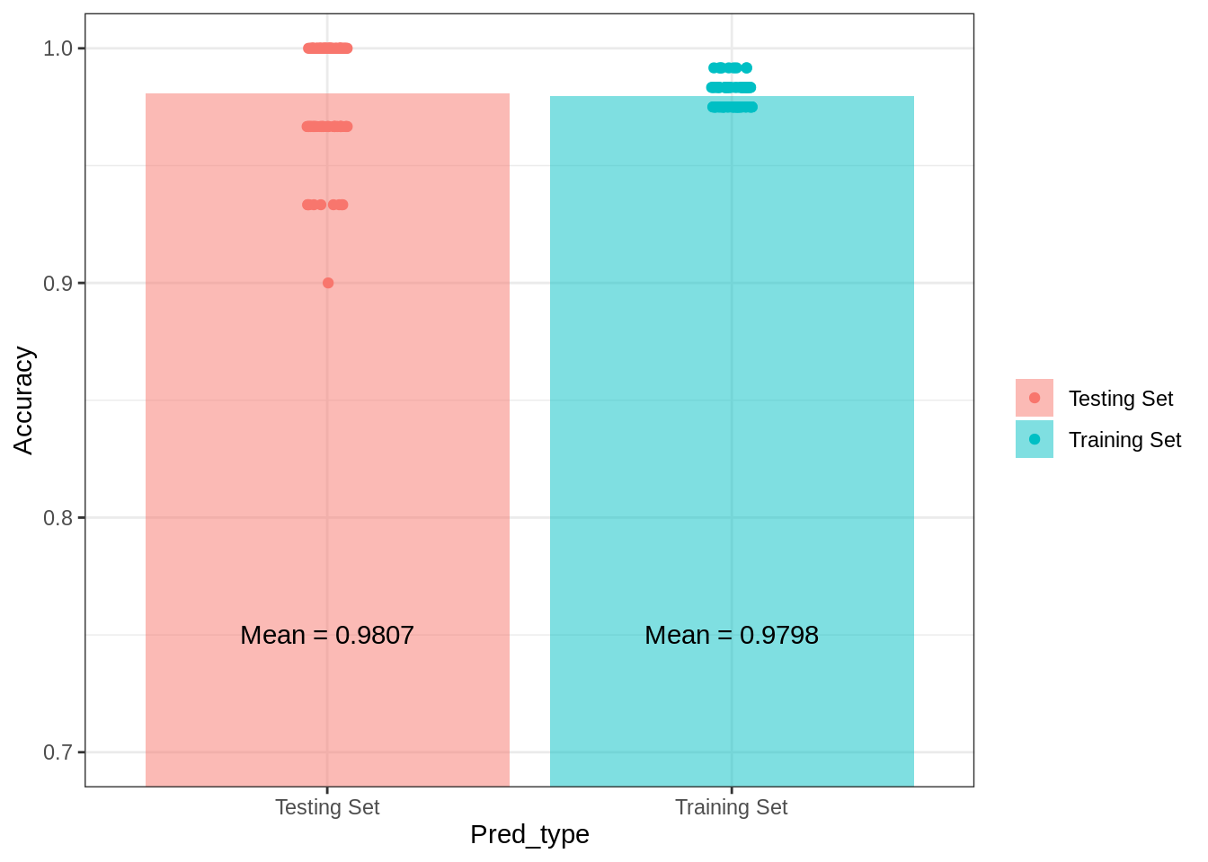
Now, whether you believe this model is a statistical model or a machine learning model, it is clear that it outperforms the Naive Bayes classifier, making more accurate in- and out-of-sample predictions in the current data set. The variance in prediction accuracy is also much smaller with this modeling approach. As with the Naive Bayes model, I included, the complete in-sample confusion matrix using a linear discriminant analysis below.
LDA_full<-lda(Species~., data=iris)
LDA_full_pred<-predict(LDA_full)$class
table(LDA_full_pred, iris$Species)
##
## LDA_full_pred setosa versicolor virginica
## setosa 50 0 0
## versicolor 0 48 1
## virginica 0 2 49The pattern of errors is slightly different than the mixture-model discriminant analysis at the end of the first post, but the overall in-sample results are the same. Each technique resulted in a total of 3 misclassifications.
Multinomial logistic regression
I will be switching up the data sets in the next post so that I can compare some more traditional machine learning/artifical intelligence approaches to basic statistical models, and when I do, I will use a binomial logistic regression as one of the models. I only say that to highlight the fact that I am presenting a multinomial logistic regression (which is essentially a series of binomial logistic regressions) before I provide information about logistic regression foundations, which I will detail more in the next post (I’ll add a link here once it is complete).
For now, know that a multinomial logistic regression is an extension of binomial or binary logistic regression. These models attempt to predict the log odds of an event occurring (also known as the logits).
\[log\Big(\frac{P(y)}{1-P(y)}\Big)=\beta_0+\beta_1X_1+\beta_2X_2+...\beta_pX_p+\epsilon\]
This link function is one of several that form the basis of what are referred to as generalized linear models. This class of models allows analysts to predict, via linear combinations of predictors (as is the case with linear regression), outcomes that do not result in normal distributions of model-based residuals. Normality of residuals is a statistical property assumed by ordinary least squares regression, which works through minimizing the total error.
Using a special case of a generalized linear model, the multinomial logistic regression, let’s go ahead and attempt to predict Species as we have done so many times before. A quick note, the function I am using to create a logistic regression model comes from the nnet package.
data("iris")
set.seed(321)
k.fold<-100
library(nnet)

#Setting up a series of vectors for tracking accuracy
Start<-Sys.time()
Accuracy<-vector()
Model<-vector()
Pred_type<-vector()
for(i in 1:k.fold){
  #Split data into training/testing set
  smpl_size<-floor(.8*nrow(iris))
  ind <- sample(seq_len(nrow(iris)), size = smpl_size)
  train<-iris[ind, ]
  test<-iris[-ind, ]

  #Train the model and obtain accuracy based on observed data
  MLR_train<-multinom(Species~., data=train, trace=FALSE)
  #note the inclusion of $class here - the way an lda object is stored
  MLR_train_pred<-predict(MLR_train, newdata = train)
  tab_train<-table(MLR_train_pred, train$Species)
  Train_acc<-sum(diag(tab_train))/nrow(train)
  Accuracy<-c(Accuracy, Train_acc)
  Model<-c(Model, 'MLR')
  Pred_type<-c(Pred_type, 'Training Set')

  #Test model and get out of sample accuracy
  MLR_test_pred<-predict(MLR_train, newdata = test)
  tab_test<-table(MLR_test_pred, test$Species)
  Test_acc<-sum(diag(tab_test))/nrow(test)
  Accuracy<-c(Accuracy, Test_acc)
  Model<-c(Model, 'MLR')
  Pred_type<-c(Pred_type, 'Testing Set')
}
round(Sys.time()-Start, digits = 2)
## Time difference of 0.57 secsOnce again a fairly quick run time (by the way I keep saying this because I am used to waiting a few hours for multilevel Bayesian regression models with correlated random effects to coverge. Waiting a second or two to get aggregated results is nothing).
Let’s see the prediction results…
MLR_KFold<-data.frame(Accuracy = Accuracy,
                     Model = Model,
                     Pred_type = Pred_type)

g1<-ggplot(data=MLR_KFold, aes(x=Pred_type, y=Accuracy))+
  geom_bar(aes(fill=Pred_type),
           alpha=.5,
           stat='summary',
           fun.y='mean')+
  geom_point(aes(color=Pred_type),
             position = position_jitter(w = 0.05, h = 0))+
  coord_cartesian(ylim=c(.70, 1))+
  guides(fill=guide_legend(title=""),
         color=guide_legend(title = ""))+
  annotate(geom='text', x = 1, y = .75,
           label = paste('Mean =',
                         round(mean(MLR_KFold$Accuracy[Pred_type=='Testing Set']),
                                         digits = 4)))+
  annotate(geom='text', x = 2, y = .75,
           label = paste('Mean =',
                         round(mean(MLR_KFold$Accuracy[Pred_type=='Training Set']),
                                         digits = 4)))+
  theme_bw()
## Warning: Ignoring unknown parameters: fun.yg1## No summary function supplied, defaulting to `mean_se()`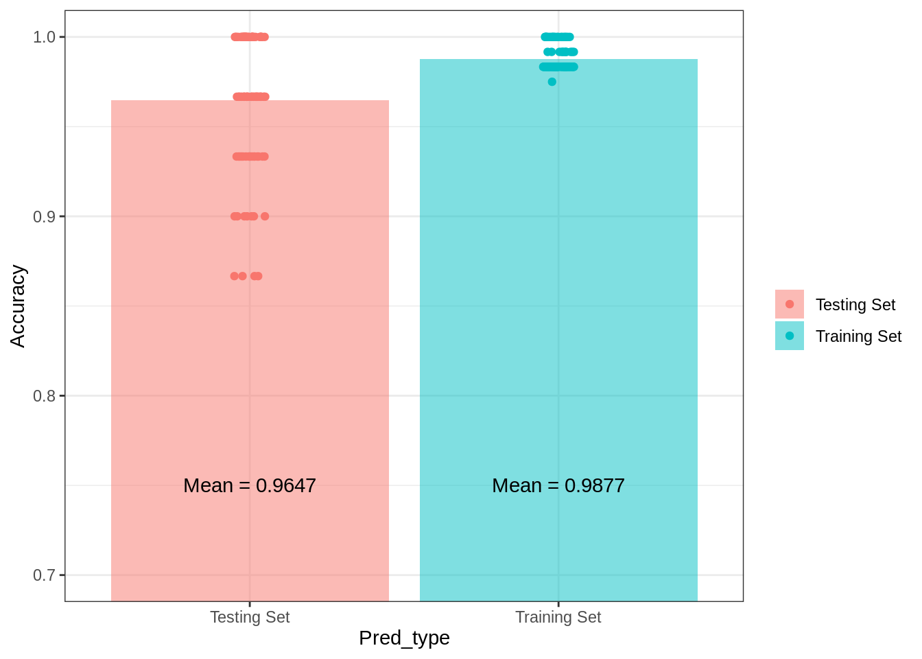
Interestingly, compared to the Naive Bayes model, the multinomial logistic regression performs better in-sample. However, there is a larger dropoff in this model’s in-sample versus out-of-sample predictive accuracy. Additionally, the results indicate that cross-validated variability in predictive accuracy is about as variable as the Naive Bayes model. If I were considering these three models for a prediction task related to these data, so far the linear discriminant model is the best.
The next post will delve into additional modeling approaches using a new dataset. Where possible these same models covered using the iris data set will also be applied to compare their predictive performance under the same set of data conditions.
References
Gelman, Andrew, and Jennifer Hill. 2007. Data Analysis Using Regression and Multilevel/Hierarchical Models. Cambridge Press.
Zumel, Nina, and John Mount. 2014. Practical Data Science with R. Manning Publications.