By Matthew Barstead | August 16, 2018
It is official. The program I have spent the better part of a year working on, the very centerpiece of my dissertation, works. Or at least, early indicators are in, and based on 22 cases, some of which required a great deal of manual editing, the program is returning estimates in line with expectations.
Backing up, as I trip a little over my excitement, IBI VizEdit is an Rshiny application I created to help the Laboratory for the Study of Child and Family Relationships process and edit heart rate data. We used a photoplethysmogram to measure changes in light absorption in a local capillary bed, in this case the child’s fingertip. As blood flows through the capillary bed in sync with the beating heart, the amount of light absorbed by the underlying tissue varies, particularly within certain wavelengths. With this knowledge and a sufficiently high sampling rate (we used 2000 Hz), you can readily record heart beats using a relatively low-cost sensor.
Individual heart rate data contains a surprising amount of information that can be used to predict an individual’s cognitive and affective states as well as predict global mental and physical health outcomes. Paired with specific tasks, we can get a sense of how effective the autonomic nervous system is at regulating internal states that are designed to potentiate certain response patterns (i.e., fleeing, fighting, freezing, behaviors).
Currently, there are no open-source tools available to researchers interested in measures of heart-rate variability obtained via photoplethysmography. That is why I created IBI VizEdit. It is still very much in its early in its lifecycle and it will be re-factored considerably in the coming months. The pogram is primarily designed to work with our Laboratory for the Study of Child and Family Relationship’s files in ways that optimize output for what we plan to do with the data. I eventually plan to adapt the program to be more general in its input to allow researchers to upload files of just about any basic data format (e.g., .dat, .txt, csv, etc.).
For now, I am just happy to be getting off on the right foot. And here are (again to be stressed) the preliminary results of an analysis of 22 edited cases. Participants in the study experienced three conditions during a baseline laboratory visit. The first is a child-appropriate Sesame Street video, which the child sees three times. In addition to the videos children also experienced two stressors: the appearance of a clown and the recording of an introduction video. The sixth task (fourth in its presentation) was a social attention task in which children learned about fictitious children and their interests.
Now if the program is working, estimates based on its output should show that respiratory sinus arrhythmia (RSA) is lowest during the Clown and Introduction tasks and highest during the Video and social attention (Kids) tasks.
So what do we find… First always graph your data. I really like the sideways raincloud plot (or nose plot) as an option for plotting. It sort of puts all of your data out there for everyone to see.
First let’s look at the RSA values by task:
df.m<-reshape2::melt(dat.RSA[,2:7])

g1<-ggplot(data = df.m, aes(y = value, x = variable, fill=variable)) +
  geom_flat_violin(position = position_nudge(x = .2, y = 0), alpha = .8) +
  geom_point(aes(y = value, color = variable),
             position = position_jitter(width = .15),
             size = .5, alpha = 0.8) +
  geom_boxplot(width = .1, guides = FALSE, outlier.shape = NA, alpha = 0.5) +
  expand_limits(x = 5.25) +
  scale_color_brewer(palette = "Dark2") +
  scale_fill_brewer(palette = "Dark2") +
  theme_bw() +
  raincloud_theme+
  xlab('')+ylab('RSA')+
  guides(fill=FALSE, color=FALSE)+
  ggtitle('Distribution of Respiratory Sinus Arrhythmia as a Function of Task')
g1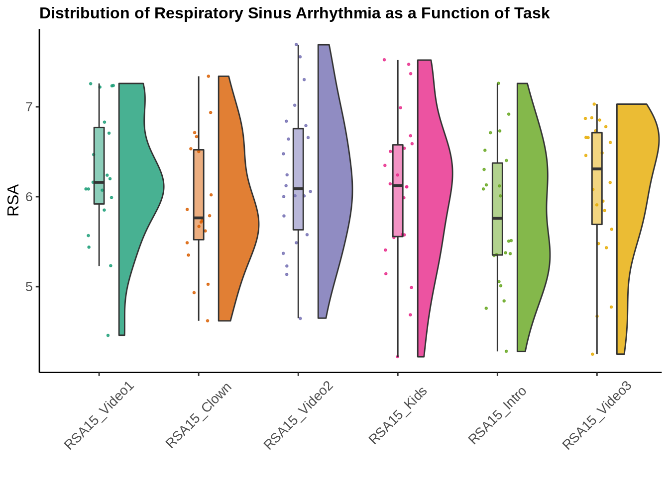
So a good amount of spread, but even with only 22 cases we can start to see the expected pattern. The medians for the videos and the social attention tasks (Kids) are higher than the median RSA values for the two distressing tasks.
I would expect heart period (the inverse of heart rate - think the time, in seconds, between successive beats) to show a similar pattern.
df.m<-reshape2::melt(dat.HP[,2:7])

g2<-ggplot(data = df.m, aes(y = value, x = variable, fill=variable)) +
  geom_flat_violin(position = position_nudge(x = .2, y = 0), alpha = .8) +
  geom_point(aes(y = value, color = variable),
             position = position_jitter(width = .15),
             size = .5, alpha = 0.8) +
  geom_boxplot(width = .1, guides = FALSE, outlier.shape = NA, alpha = 0.5) +
  expand_limits(x = 5.25) +
  scale_color_brewer(palette = "Dark2") +
  scale_fill_brewer(palette = "Dark2") +
  theme_bw() +
  raincloud_theme+
  xlab('')+ylab('HP')+
  guides(fill=FALSE, color=FALSE)+
  ggtitle('Distribution of Heart Period as a Function of Task')

g2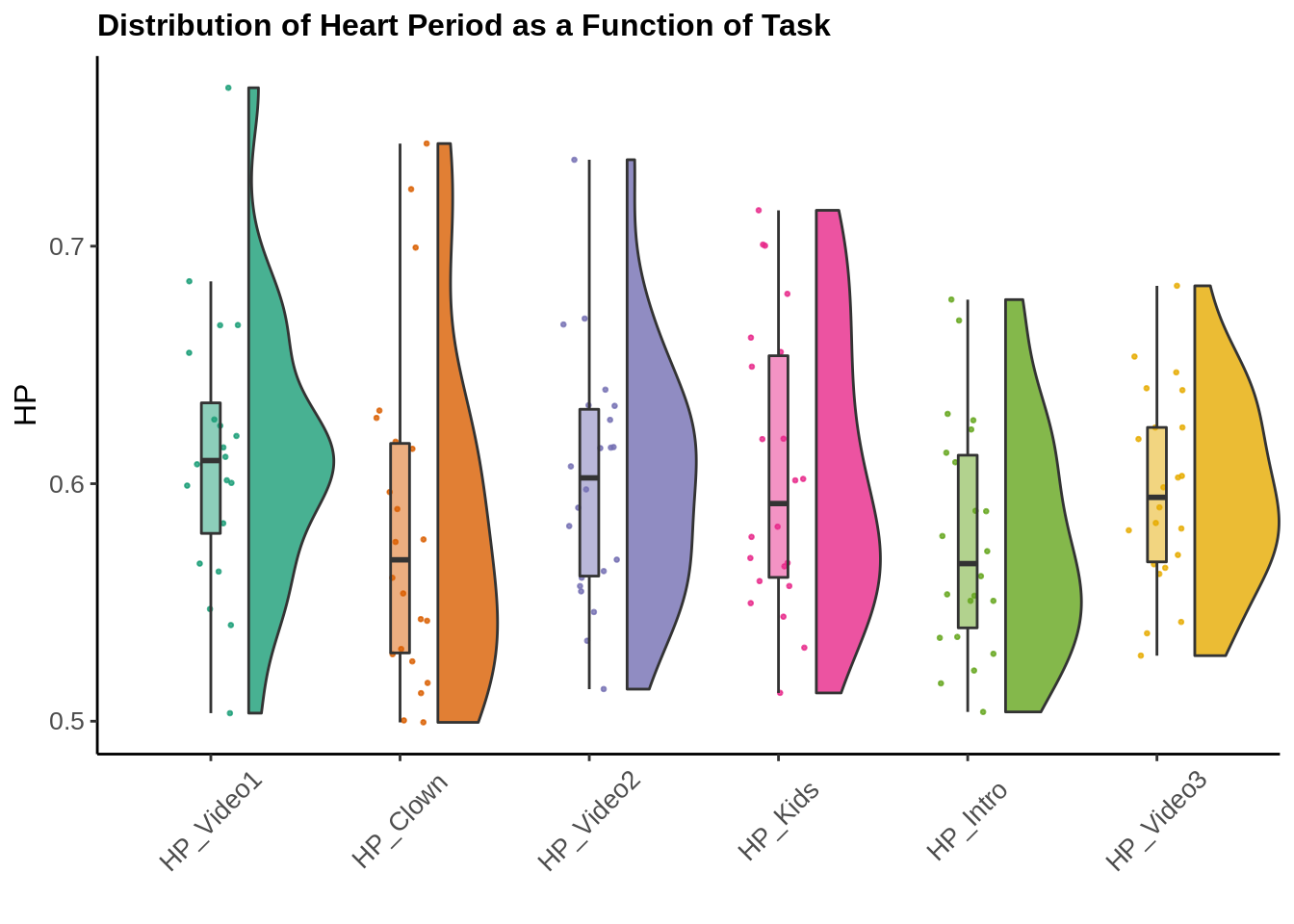
Lo and behold largely the same pattern. This is good for me so far. So let’s see if it passes an inferential test. Do the two distressing tasks each reliably depress heart rate variability (in the form of respiratory sinus arrhythmia) and average heart period?
#--
fit.RSA<-lmer(RSA~1+Clown+Video2+Kids+Intro+Video3+(1|File),
                data=dat.RSA.long)
summary(fit.RSA)
## Linear mixed model fit by REML ['lmerMod']
## Formula: RSA ~ 1 + Clown + Video2 + Kids + Intro + Video3 + (1 | File)
## Data: dat.RSA.long
##
## REML criterion at convergence: 208.6
##
## Scaled residuals:
## Min 1Q Median 3Q Max
## -2.13205 -0.68779 -0.00623 0.52208 2.77992
##
## Random effects:
## Groups Name Variance Std.Dev.
## File (Intercept) 0.4429 0.6655
## Residual 0.1801 0.4244
## Number of obs: 125, groups: File, 22
##
## Fixed effects:
## Estimate Std. Error t value
## (Intercept) 6.18134 0.17278 35.776
## Clown -0.30111 0.14211 -2.119
## Video2 0.03093 0.13383 0.231
## Kids -0.10134 0.13383 -0.757
## Intro -0.38043 0.13383 -2.843
## Video3 -0.08134 0.13383 -0.608
##
## Correlation of Fixed Effects:
## (Intr) Clown Video2 Kids Intro
## Clown -0.399
## Video2 -0.420 0.515
## Kids -0.420 0.515 0.543
## Intro -0.420 0.515 0.543 0.543
## Video3 -0.420 0.515 0.543 0.543 0.543#Getting bootstrapped CIs for model results
boot.RSA<-bootMer(fit.RSA, fixef, nsim=5000)
print(sjstats::boot_ci(boot.RSA))## term conf.low conf.high
## 1 X.Intercept. 5.8469298 6.51271477
## 2 Clown -0.5802894 -0.02298513
## 3 Video2 -0.2267125 0.29510555
## 4 Kids -0.3658046 0.16269253
## 5 Intro -0.6388097 -0.11533016
## 6 Video3 -0.3395032 0.18322587Looking at the estimated t-scores, and my prefered method - the boot-strapped confidence interval, we see much the same story. RSA estimates were reliably lower during the clown and video introduction task relative to the first video (there were no other significant differences).
#--
fit.HP<-lmer(HP~1+Clown+Video2+Kids+Intro+Video3+(1|File),
                data=dat.HP.long)
summary(fit.HP)
## Linear mixed model fit by REML ['lmerMod']
## Formula: HP ~ 1 + Clown + Video2 + Kids + Intro + Video3 + (1 | File)
## Data: dat.HP.long
##
## REML criterion at convergence: -489.2
##
## Scaled residuals:
## Min 1Q Median 3Q Max
## -2.7645 -0.5346 0.0340 0.5869 3.5147
##
## Random effects:
## Groups Name Variance Std.Dev.
## File (Intercept) 0.002568 0.05068
## Residual 0.000554 0.02354
## Number of obs: 130, groups: File, 22
##
## Fixed effects:
## Estimate Std. Error t value
## (Intercept) 0.6061055 0.0120385 50.347
## Clown -0.0240009 0.0073053 -3.285
## Video2 -0.0049964 0.0073053 -0.684
## Kids -0.0008464 0.0073053 -0.116
## Intro -0.0296282 0.0073053 -4.056
## Video3 -0.0089237 0.0073053 -1.222
##
## Correlation of Fixed Effects:
## (Intr) Clown Video2 Kids Intro
## Clown -0.320
## Video2 -0.320 0.528
## Kids -0.320 0.528 0.528
## Intro -0.320 0.528 0.528 0.528
## Video3 -0.320 0.528 0.528 0.528 0.528#Getting bootstrapped CIs for model results
boot.HP<-bootMer(fit.HP, fixef, nsim=5000)
print(sjstats::boot_ci(boot.HP))## term conf.low conf.high
## 1 X.Intercept. 0.58266382 0.629469814
## 2 Clown -0.03823164 -0.009566613
## 3 Video2 -0.01921925 0.009463821
## 4 Kids -0.01504550 0.013696701
## 5 Intro -0.04381934 -0.015358019
## 6 Video3 -0.02332425 0.005673628And the pattern was replicated with heart period.
I definitely do not want to oversell these results. They are just a good sign is all as I continue to finalize this program and its features.