By Matthew Barstead, Ph.D. | May 21, 2018
(Updated: 2020-12-31)
Problem Statement
Create a forecast model using only the information available in a single, univariate time series.
The Past is Prologue
Sometimes the only data we have to predict a particular phenomenon are previous measurements of the target variable we hope to forecast. Using the past to predict the future means that we assume prior trends will continue into the forecast window. Absent other information and all else being equal, making a past is prologue assumption is not a terrible decision in many cases.
If we can reasonably talk ourselves into making this assumption, then a number of modeling approaches become viable. Among the simplest techniques would be something like a linear regression. Despite its simplicity, there are many processes for which the only reliable pattern over time is a consistent, linear change.
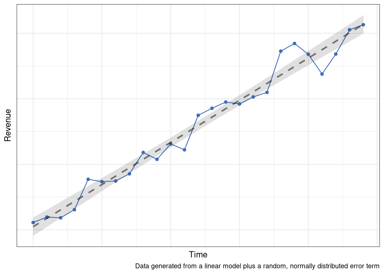
More likely though, the true data generation process is going to be the sum of multiple patterns or processes over time.
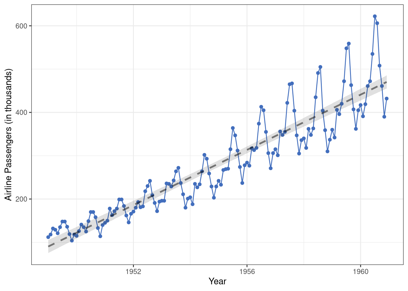
For example, following properties of this second time-series (monthly airline passengers from 1949-1960) stand out, only one of which can be accounted for by a linear change process.
- There is an average trend over time.
- There is a seasonal trend.
- As time progresses the seasonal trend becomes stronger…
- … and the variation in monthly airline passengers increases
For the remainder of the post we are going to focus on creating a Gaussian process forecast model from these data. We’ll use the data set to define a set of functions we think can be used to model the co-variance between two observations over time. See the “Deeper Dive: GP Models are the Sum of Their Parts” box below if you are interested more details. Otherwise, feel free to skip ahead to the Modeling Walkthrough.
Deeper Dive: GP Models are the Sum of Their Parts
Gaussian process models encompass an incredibly flexible modeling framework. One reason for this flexibility is that the sum of any number of Gaussian processes is a Gaussian process. What this means in practice is that we can layer multiple processes on top of one another in our model. So if we think there is an average change component - we can include a process that accounts for linear change. If we think there are additional patterns - we can add those processes as well.
So how does it all work? Well, a Gaussian process model is a series of mean and co-variance functions that we think give rise to the data. Most of the action is in the co-variance functions (called kernels) that are implied by each process. This fact is both a bit of a blessing and a curse at the same time. On the one had, it is convenient that we can string together multiple processes and aggregate their contributions to forecasting future events in a principled way. After all, most outputs we want to model are multiply caused. On the other hand, the computational resources required to implement these models is prohibitive, which can make problems involving very large data sets practically intractable.
The computational burden is the result of needing to take the determinant and the inverse of the co-variance matrix, and in a Bayesian context this expensive calculation has to take place with each draw from the posterior. The upshot is that these models are \(O(N^3)\) efficient. So we are definitely paying a cost for our flexibility. I personally believe these models have value even when used in “Bid Data” contexts, provided the implementer works to make the computational and modeling steps as efficient as possible (e.g., downsample, save and use parameters not entire distributions, etc.).
For additional reading, the definitive text on this modeling family as far as I know is Rasmussen and Williams (2006). David Duvenaud put together a nice little webpage that has a good overview of different co-variance functions and how to combine them. A good thread on covariance functions and how they work their magic is available on Cross Validated.
Modeling Walkthrough
Gaussian process models are a form of supervised learning in that the analyst has to define one or more co-variance functions to account for the data. We start by using a model to identify some set of maximally likely parameters for each function (or in a Bayesian context a distribution of parameters). Some modelers refer to this phase as “tuning” the hyperparameters. When the hyperparameters are sufficiently tuned, we take the co-variance functions and the hyperparameters and feed in a time window outside the data used for training the model (typically after the training data in time, but sometimes we are interested in “backcasting”).
The modeling process may sound straightforward. But it isn’t always. Building a good Gaussian process model (well, really any model) requires a bit of iteration. Along the way, the analyst selects which kernels to add or multiply together to try to reliably re-create the patterns observed in the historical data. Making these choices is a mix of trial and error, statistical reasoning, and muttered curse words.
Example: Say we worked for “Big Ice Cream” and we wanted to know, using our own sales records, our expected sales for the upcoming year? Being in the business of selling ice cream and ice cream accessories for so many years, we know there is a reliable pattern that unfolds annually. Our lowest sales are the winter months. We ramp up through the spring, peak in the summer, and start to return back down to the lower winter levels in the fall. We also know that ice cream sales in general are up over the past few years. The first process suggests there is a detectable annual cycle that peaks each summer. A periodic kernel of some sort should be able to capture a pattern that repeats reliably over time. The second process suggests that over time values are going up. We could either use a linear kernel (though there may be more efficient ways to achieve the same end), or a simple “decay” kernel like the squared exponential co-variance kernel. Modeling the
AirPassengersdata will involve both a periodic kernel and a squared exponential kernel (in several capacities).
Modeling Overview
In terms of modeling strategy, we’ll start with a simple, common co-variance function - the squared exponential kernel. From there we’ll explore possible transformations and additional kernels. We’ll be using the AirPassengers data that ships with R. For more information about the data type ?AirPassengers in your R terminal.
The goal here is to build a forecast model that yields our best guess of future monthly airline passengers, given the trends we’ve seen over the preceding 10-year period. So how do we know if our model is any good? Since we can’t test the model’s performance against the future outcomes when building it, we’ll do the next best thing - split the data into a training epoch and a testing epoch. The training epoch is for tuning the model’s hyperparameters on historical data. The testing epoch is a “mock” forecast of sorts. We’re basically saying, what if we had used this model in 1959 - using all the data available up to that point - to predict monthly passengers in 1960? How well would the model have done? Absent a crystal ball, playing out this counterfactual forecasting scenario will be one of our best tests of the effectiveness of the model.
Before modeling we split out the training (1949-1959) and testing (1960) data.
air_pass_train <- air_pass_tbl %>%
  filter(year < 1960)

air_pass_test <- air_pass_tbl %>%
  filter(year >= 1960)
Model 1
As mentioned above, the first model will use the squared exponential co-variance function (below) as the sole Gaussian process.
\[k(t,t') = \sigma^2 exp\Big(-\frac{(t-t')^2}{2l^2}\Big)\]
We’re interested in tuning the “length” parameter \(l^2\) and the variance parameter \(\sigma^2\) of this co-variance function. The length parameter governs how strongly correlated two points are as a function of time. The \(\sigma^2\) parameter “weights” or “scales” this function’s contribution to the overall co-variance matrix.
Let’s get the data ready:
m1_data <- list(
  N1 = nrow(air_pass_train),
  N2 = nrow(air_pass_test),
  X = air_pass_train[['year']],
  Y = air_pass_train[['pass']],
  Xp = air_pass_test[['year']]
)
The model variables are:
N1: the number of observations in the training setN2: the number of observations in the test setX: evenly spaced interval of time in the training setY: passengers in a given month in the training setXp: evenly spaced interval of time in the test set
I was inspired by and borrowed from Nate Lemoine’s post on Gaussian processes when setting this model up. I highly recommend his posts if you are interested in gaining additional exposure to this modeling technique.
functions{
    //covariance function for main portion of the model
    matrix main_GP(
        int Nx,
        vector x,
        int Ny,
        vector y,
        real alpha1,
        real rho1){
                    matrix[Nx, Ny] Sigma;

                    //specifying random Gaussian process that governs covariance matrix
                    for(i in 1:Nx){
                        for (j in 1:Ny){
                            Sigma[i,j] = alpha1*exp(-square(x[i]-y[j])/2/square(rho1));
                        }
                    }

                    return Sigma;
                }
    //function for posterior calculations
    vector post_pred_rng(
        real a1,
        real r1,
        real sn,
        int No,
        vector xo,
        int Np,
        vector xp,
        vector yobs){
                matrix[No,No] Ko;
                matrix[Np,Np] Kp;
                matrix[No,Np] Kop;
                matrix[Np,No] Ko_inv_t;
                vector[Np] mu_p;
                matrix[Np,Np] Tau;
                matrix[Np,Np] L2;
                vector[Np] yp;

    //--------------------------------------------------------------------
    //Kernel Multiple GPs for observed data
    Ko = main_GP(No, xo, No, xo, a1, r1);
    for(n in 1:No) Ko[n,n] += sn;

    //--------------------------------------------------------------------
    //kernel for predicted data
    Kp = main_GP(Np, xp, Np, xp,  a1, r1);
    for(n in 1:Np) Kp[n,n] += sn;

    //--------------------------------------------------------------------
    //kernel for observed and predicted cross
    Kop = main_GP(No, xo, Np, xp,  a1, r1);

    //--------------------------------------------------------------------
    //Algorithm 2.1 of Rassmussen and Williams
    Ko_inv_t = Kop'/Ko;
    mu_p = Ko_inv_t*yobs;
    Tau=Kp-Ko_inv_t*Kop;
    L2 = cholesky_decompose(Tau);
    yp = mu_p + L2*rep_vector(normal_rng(0,1), Np);
    return yp;
    }
}

data {
    int<lower=1> N1;
    int<lower=1> N2;
    vector[N1] X;
    vector[N1] Y;
    vector[N2] Xp;
}

transformed data {
    vector[N1] mu;
    for(n in 1:N1) mu[n] = 0;
}

parameters {
  // a1, r1, and sigma_sq cannot be negative
    real<lower=0> a1;
    real<lower=0> r1;
    real<lower=0> sigma_sq;
}

model{
    matrix[N1,N1] Sigma;
    matrix[N1,N1] L_S;

    //using GP function from above
    Sigma = main_GP(N1, X, N1, X,  a1, r1);
    for(n in 1:N1) Sigma[n,n] += sigma_sq;

    L_S = cholesky_decompose(Sigma);
    Y ~ multi_normal_cholesky(mu, L_S);

    // priors for parameters - effecitvely the upper half of the students t-distribution
    a1 ~ student_t(3,0,1);
    r1 ~ student_t(3,0,1);
    sigma_sq ~ student_t(3,0,1);
}

generated quantities {
    vector[N2] Ypred = post_pred_rng(a1, r1, sigma_sq, N1, X, N2, Xp, Y);
}
And now to execute this using the rstan wrapper function.
# Easier to note these upfront
m1_pars.to.monitor<-c('a1','r1','sigma_sq', 'Ypred')

# Note that I have a machine at home with 12 logical cores and 64GB of RAM
# You may want to lower the number of chains and or cores
m1 <- stan(
  file = '../../blog_code/gp_m1.stan',
  data = m1_data,
  warmup = 1000,
  iter = 2000,
  refresh=1000,
  chains = 6,
  pars = m1_pars.to.monitor,
  control = list(adapt_delta = .95,
                 max_treedepth = 10),
  seed = 20030414
)
The model will converge, though there is some evidence that not all is well. I see a lot of warnings like the one below that make me think there is some kind of numerical instability causing problems. Given how close the values are, this has all of the elements of a floating point precision problem.
Exception: Exception: cholesky_decompose: m is not symmetric. m[1,3] = 61.9907, but m[3,1] = 61.9917 (in 'model6e5051823be5_gp_m1' at line 59)
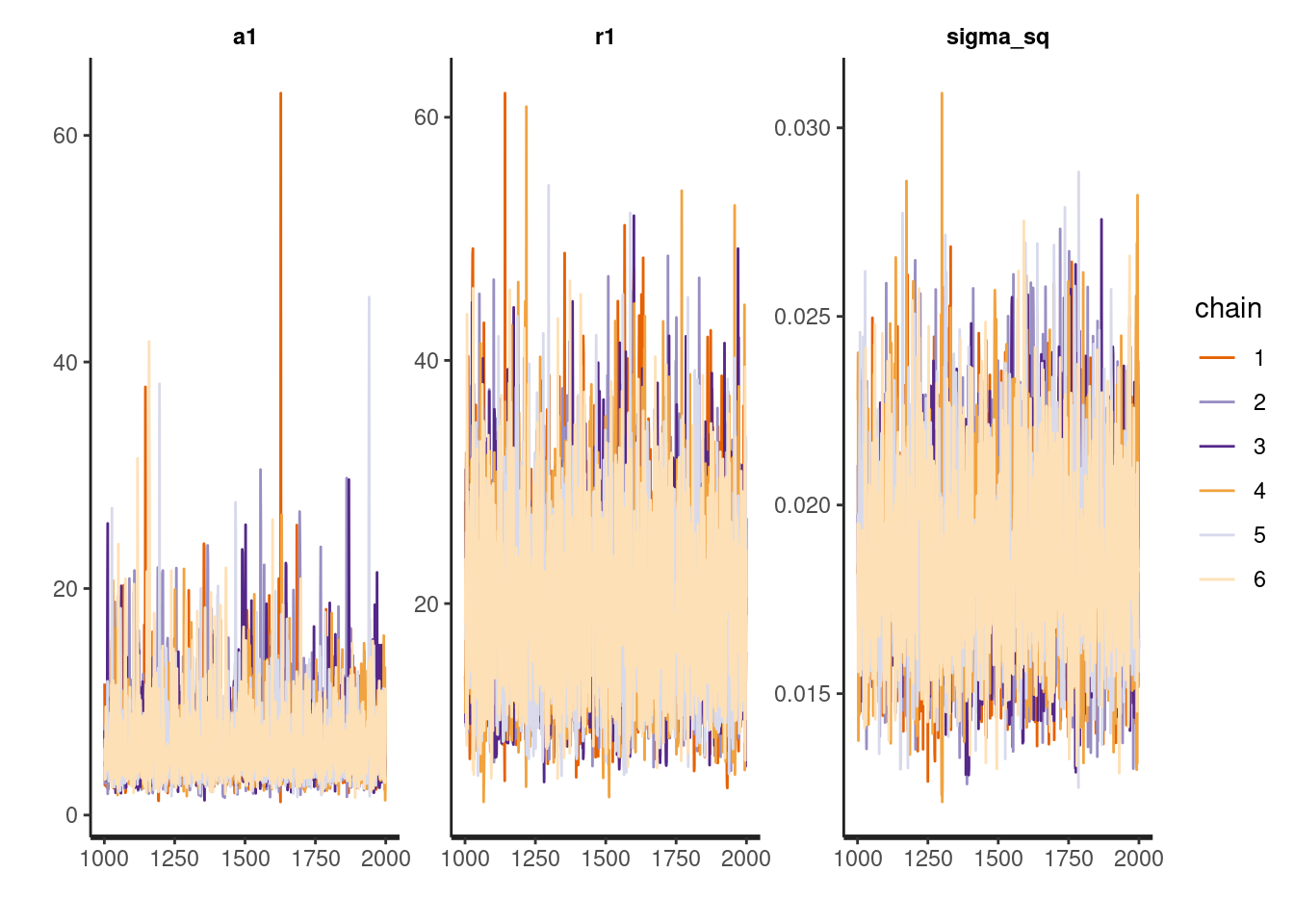
(in 'model6e5051823be5_gp_m1' at line 103)Despite the seeming instability, the trace plots below suggest the distributions of the model parameters converged reasonably well (a few spikes I don’t love). I often use more chains when model building to help with diagnosis problems if they arise. Three chains should be sufficient for diagnosing most model problems. I use 6 because I am working on a 12-core machine and I can.
traceplot(m1, pars=c('a1', 'r1', 'sigma_sq'))
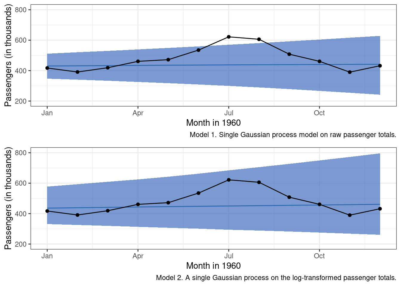
In terms of forecast performance, the predictions don’t seem to have a way of accounting for the non-linear annual cycle at all.
g_m1 <-
brms::posterior_samples(m1, 'Ypred') %>%
  as.data.frame() %>%
  pivot_longer(cols = starts_with('Ypred'), values_to = 'pass') %>%
  mutate(
    year = rep(air_pass_test[['year']], 6000)
  ) %>%
  ggplot(aes(x = year, y = pass)) +
  stat_lineribbon(color = "#08519C", fill = '#426EBD', lwd = .5, .width = .95, alpha = .7) +
  geom_point(data = air_pass_test, aes(x = year, y = pass)) +
  geom_line(data = air_pass_test, aes(x = year, y = pass)) +
  labs(x = "Month in 1960", y = "Passengers (in thousands)",
       caption = 'Model 1. Single Gaussian process model on raw passenger totals.') +
    scale_x_continuous(breaks = c(1960, 1960.25, 1960.5, 1960.75),
                     labels = c('Jan', 'Apr', 'Jul', 'Oct')) +
  theme_bw()

g_m1
We can do better.
Model 2
One initial concern with the first Gaussian process model I have is the potential floating point precision problems indicated by the Stan Exceptions thrown. One possible cause is a mismatch of scales - that is, over time, mean values and variation are becoming much larger. A common solution is to log-transform time-series in these instances. The model is still going to predict total airline passengers. We are just going to be modeling the change in terms of log-units or “magnitude” units, and then exponentiate back across our log link function to get predictions back in the original scale.
All we have to do is change our transformed data block as so in our Stan model:
transformed data {
    vector[N1] mu;
    vector[N1] y_log;
    for(n in 1:N1){
      mu[n] = 0;
      y_log[n] = log(Y[n]);
    }
}
And add y_log in where appropriate:
model {
    matrix[N1,N1] Sigma;
    matrix[N1,N1] L_S;
  ...
  y_log ~ multi_normal_cholesky(mu, L_S);
  ...
}

generated quantities {
    vector[N2] Ypred = post_pred_rng(a1, r1, sigma_sq, N1, X, N2, Xp, y_log);
}
With the transform added we can re-run our model with the single squared exponential co-variance function.
# Model is the same in terms of parameters - just transformed the variable to log space
m2_pars.to.monitor <- m1_pars.to.monitor

m2 <- stan(
  file = '../../blog_code/gp_m2.stan',
  data = m1_data,
  warmup = 1000,
  iter = 2000,
  refresh=1000,
  chains = 6,
  pars = m2_pars.to.monitor,
  control = list(adapt_delta = .95,
                 max_treedepth = 10),
  seed = 20030414
)
The first good news is that there are no Exceptions thrown, which is always a welcome sign, and the model seems to converge without much issue. We still see the odd spike for a1 - something worth investigating - perhaps tightening the priors would help or maybe increasing the warmup phase.
And now for a model comparison: raw vs. log-transformed.
summary_stats <- c('mean', 'sd', '2.5%', '97.5%')
summary(m1)$summary[m2_pars.to.monitor[-4], summary_stats]
## mean sd 2.5% 97.5%
## a1 27986.228803 17925.451519 9935.276868 72792.17720
## r1 6.635905 2.082673 3.555862 11.37888
## sigma_sq 1652.365847 205.829914 1293.915070 2099.19692As you can see, the scales for the parameters tuned with the first model are wildly different from one another.
summary(m2)$summary[m2_pars.to.monitor[-4], summary_stats]## mean sd 2.5% 97.5%
## a1 6.41991908 3.657668327 2.47754727 15.67998784
## r1 19.46080509 7.563883388 8.21869776 36.82942299
## sigma_sq 0.01852511 0.002394635 0.01434739 0.02379413The scales for our kernel hyperparameters are much more similar in the second model, and this approach seems to have prevented the numerical errors observed in our first model. While it is better to have addressed the Exception than to not have done so, the second model still does not perform that much better than the first.
Model 3
Visual inspection of the plots leads me to think that the log-transformed approach is maybe a little better in making predictions. But, the slight improvement is irrelevant as neither of these models is particularly good. So it looks as though we are going to need a little more cowbell. And, by cowbell I mean more co-variance functions that can encode additional patterns in the observed data. We’ll start with adding a modified periodic kernel.
\[k(t,t')=\sigma_2^2 exp\Big(-\frac{2sin^2(\pi(t-t')*1)}{l_2^2}\Big) exp\Big(-\frac{(t-t')^2}{2l_3^2}\Big)\]
Here is what it looks like when added to the main_GP function in our evolving Stan code. Note that you’ll also need to add the rho*/r* and alpha*/a* parameters in the appropriate locations throughout.
for(i in 1:Nx){
    for(j in 1:Ny){
        K2[i, j] = alpha2*exp(-2*square(sin(pi()*fabs(x[i]-y[j])*1))/square(rho2))*
        exp(-square(x[i]-y[j])/2/square(rho3));
    }
}
# Now more parameters to monitor
m3_pars.to.monitor <- c(
paste0('r', 1:3),
paste0('a', 1:2),
'sigma_sq',
'Ypred'
)
m3 <- stan(
file = '../../blog_code/gp_m3.stan',
data = m1_data,
warmup = 1000,
iter = 2000,
refresh=1000,
chains = 6,
pars = m3_pars.to.monitor,
control = list(adapt_delta = .95,
max_treedepth = 10),
seed = 20030414
)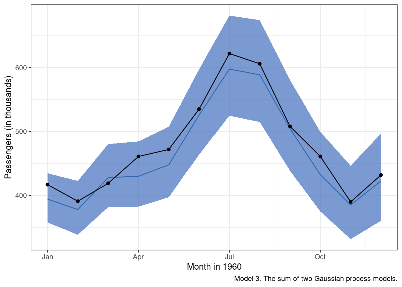
Well, that is a huge improvement over the first two models. Adding in a term that addresses the obvious seasonal pattern improved model predictions immensely. My only gripe at this point is the fact that the “mean” posterior estimate tends to undershoot the observed data on average. We’ll see if we can fix that in the next model.
Modeling Tip. We used the model posterior distributions from the second model (with the log-transformation) to define priors for our squared exponential kernel in the third model. Is that a good idea? The short answer is maybe. In the end, we want the priors to help constrain the hyperparameter space the model has to explore, but we don’t want to constrain the space to such a degree that we start to omit plausible values. Using the posteriors from one model to define the next model’s priors can be risky, as it provides a pathway for error propagation up through our model building chain. However, the payoff is that the MCMC chains may be able to be sampled more efficiently. If you want to figure out if the juice is worth the squeeze, try modifying the priors in different ways to see what sort of an impact certain changes have on run time, model accuracy and model uncertainty.
summary(m3)$summary[m3_pars.to.monitor[-7], summary_stats]## mean sd 2.5% 97.5%
## r1 25.098666623 4.727648e+00 16.984123418 34.955126986
## r2 0.722006743 1.345012e-01 0.495319899 1.023863555
## r3 21.193043675 1.000872e+01 9.272311169 46.640834126
## a1 3.884139611 8.718940e-01 2.326788426 5.728307076
## a2 0.055216350 7.678362e-02 0.010251520 0.243627906
## sigma_sq 0.001791228 2.532609e-04 0.001360783 0.002350636Model 4
Returning to the initial list of aspects we noticed when plotting the airline passenger data, let’s see what we have been able to incorporate so far.
- Over time there is an average increase in the number of passengers.
The mostly linear trend seems to be effectively captured by the first Gaussian process in the model - the squared exponential co-variance kernel.
- There is a seasonal trend on top of the average increase that appears to be annual in nature, which would make sense for the airline industry in the 1950s, with air travel peaking in July.
The properties of this seasonal trend are not necessarily constant over time, which we account for by multiplying a squared exponential kernel with a periodic kernel. This particular combination is sometimes known as a locally periodic kernel.
- The effect of the seasonal trends is more pronounced over time.
Addressed in two ways. The first is through the log-transform. The second is through the use of a locally periodic kernel (see above).
- There may, and I stress may be a slight acceleration in the long-term increase in monthly passengers.
We haven’t directly addressed this property just yet. One way to think about this component is that the decay rate in the association between two scores as a function of time is going to decay over time itself. As a result we will end up being less certain in our predictions the farther out in time they are from the observed data.
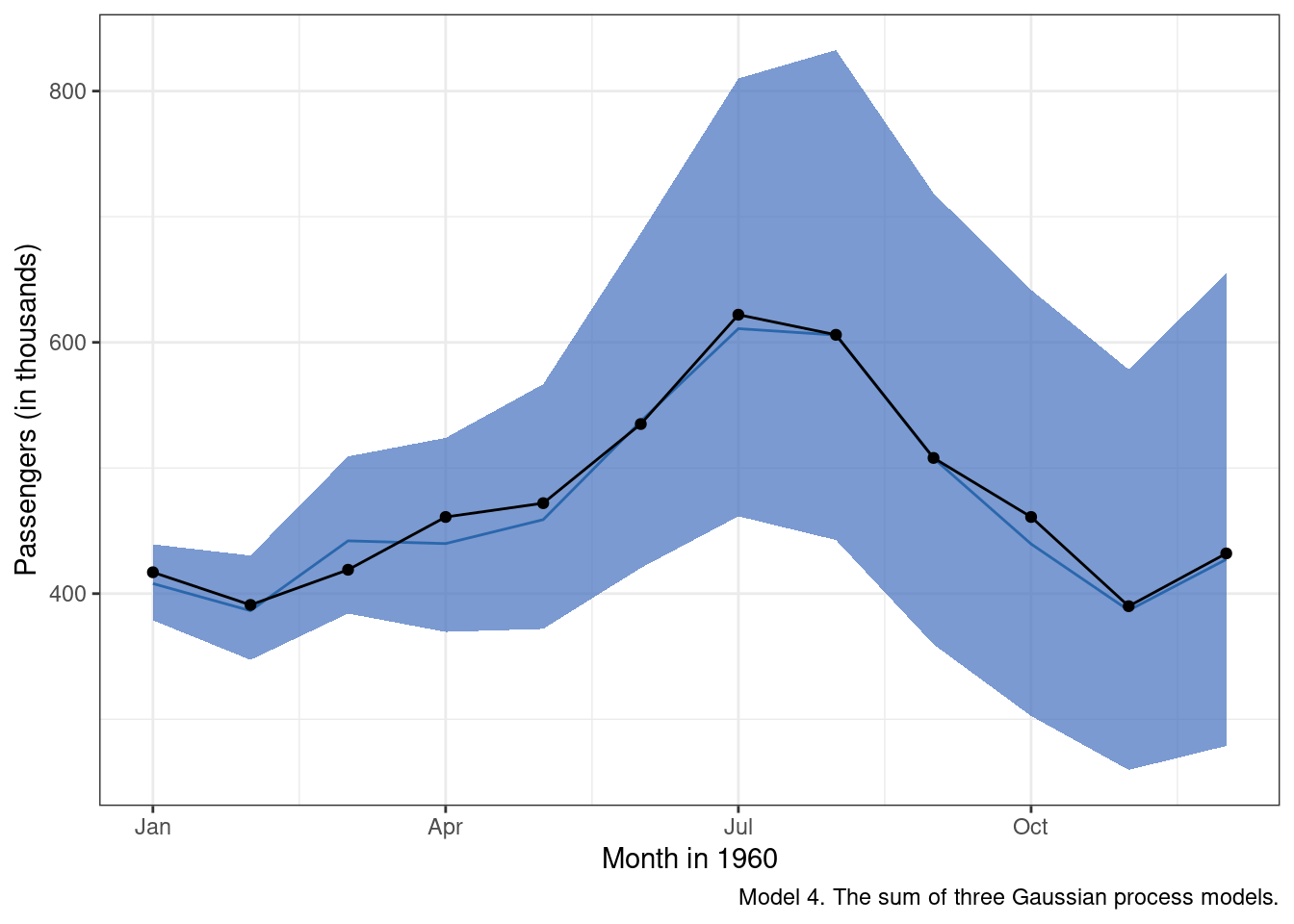
In the fourth and final model (at least for this example), I have added a third Gaussian process that enforces the concept described in #4. It is a squared exponential co-variance kernel - our good old “decay” function - multiplied by a second squared exponential kernel. Again the idea here is that the decay function is not constant. The further out we get in our forecasts, the increasingly less certain we should be about our predictions.
Deeper Dive: Kernel Functions as Weights
One way to think about kernel functions is as a series of formalized weighting systems. Each kernel function provides instructions for determining exactly how much information from data point \(x_j\) should be incorporated in data point \(x_i\) as a function of however distant \(i\) and \(j\) are. The kernel “trick” is to provide a means of modeling those weights in a functional space - dictated by the kernel selected. Different kernels imply different spaces and different weights. However, the fact that they can be added and multiplied offers nearly endless combinations of kernels to use in specifying a Gaussian process model.
Before deciding on a particular kernel, I recommend playing around a bit with different values for various kernels’ hyperparameters. Generate some of your own simulated data. Doing so will help build intuition for how changes to those values would affect expectations about observed scores.
The Stan code for generating a discontinuous time-series in which the discontinuity is caused by a change in available resources is available here. The relevant R code for generating the output is below:
pre_clip_stmts <- 1:24
post_clip_stmts <- 25:48

sim_dat <- list(
    alpha = 40,
    rho = 7,
    sigma = 2,
    N_pre = length(pre_clip_stmts),
    N_post = length(post_clip_stmts),
    x_pre = pre_clip_stmts,
    x_post = post_clip_stmts,
    mu_util = 750,
    delta_util = 125,
    icl = 1000,
    clip_amt = 500
)

sim_fit <- stan(
    file = '../../blog_code/util_sim.stan',
    data = sim_dat,
    chains = 3,
    iter = 3000,
    cores = 3,
    control = list(adapt_delta = .95, max_treedepth=15)
)
Try adjusting the delta_util term (the average change in the amount of resource utilization in raw dollars) or tinkering with the alpha or rho parameters. Mess around with the set up in the Stan code and plot your results. Look there is no reason this stuff can’t be fun… just play a little, make some statistical jazz, or at least a few wavy lines.
Armed with our third and final Gaussian process, it is time to execute this last model.
# Easier to note these upfront
m4_pars.to.monitor <- c(
  paste0('r', 1:5),
  paste0('a', 1:3),
  'sigma_sq',
  'Ypred'
)

#Note that I have a machine at home with 12 logical cores and 64GB of RAM
m4 <- stan(
  file = '../../blog_code/gp_m4.stan',
  data = m1_data,
  warmup = 1000,
  iter = 2000,
  refresh=1000,
  chains = 6,
  pars = m4_pars.to.monitor,
  control = list(adapt_delta = .95,
                 max_treedepth = 10),
  seed = 20030414
)
Inspection of the results suggests we are doing a little bit better than m3 in terms of the accuracy of the mean predicted value for each month in 1960 (the blue line). We also clearly see now that, as we get further out from the most recently observed data, there is increased uncertainty around our predictions.
And now model 4 predictions extended from the observed data:
g_m4.2 <-
brms::posterior_samples(m4, 'Ypred') %>%
  as.data.frame() %>%
  pivot_longer(cols = starts_with('Ypred'), values_to = 'pass_log') %>%
  mutate(
    year = rep(air_pass_test[['year']], 6000),
    pass = exp(pass_log)
  ) %>%
  ggplot(aes(x = year, y = pass)) +
  stat_lineribbon(color = "#08519C", fill = '#426EBD', lwd = .5, .width = .95, alpha = .7) +
  geom_point(data = air_pass_train, aes(x = year, y = pass)) +
  geom_line(data = air_pass_train, aes(x = year, y = pass)) +
  labs(x = "Year", y = "Passengers (in thousands)",
       caption = str_wrap('Model 4. Forecast: Three Gaussian process models combined')) +
  theme_bw()

g_m4.2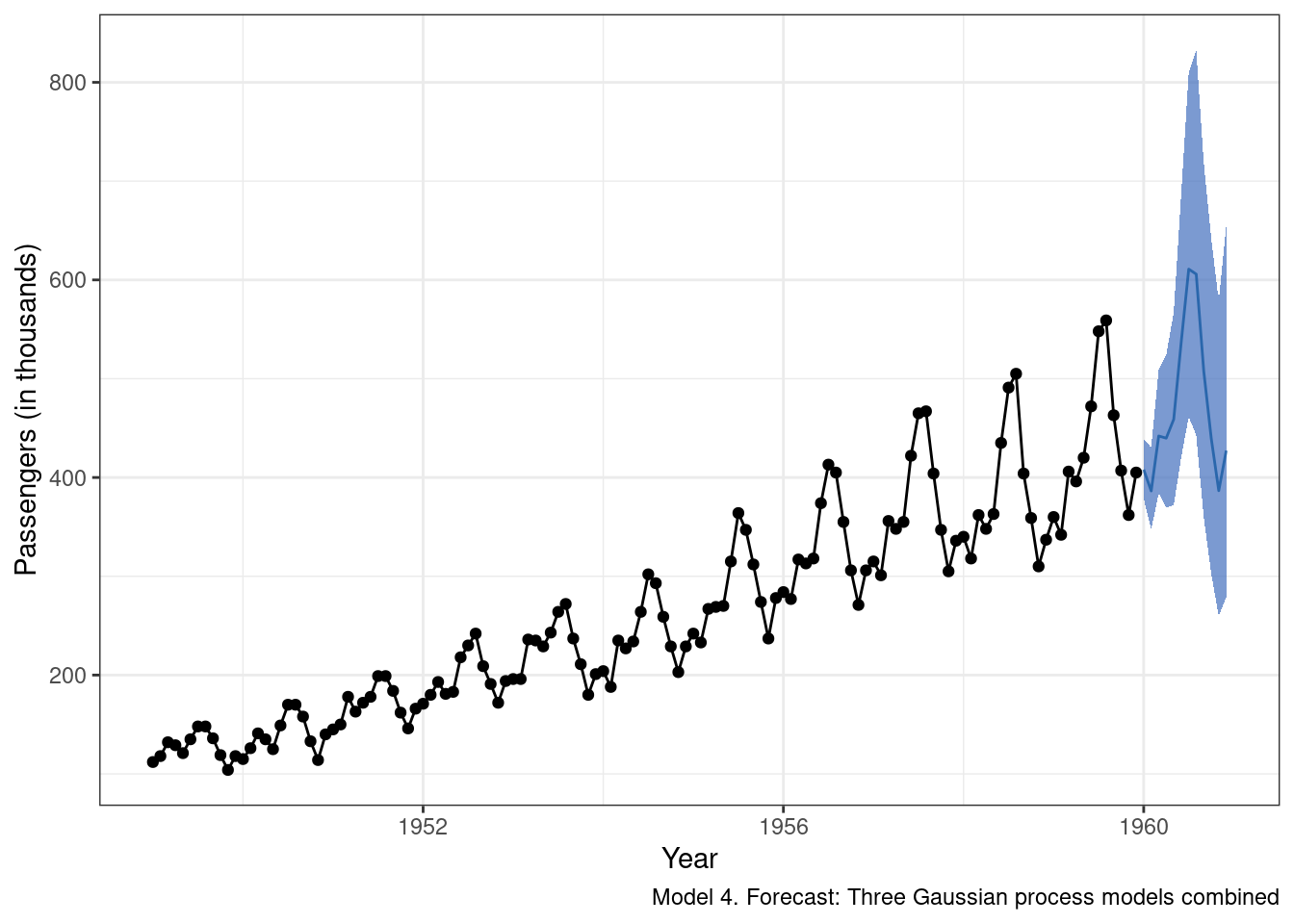
It is probably a good thing that the farther out from the observed data we attempt to forecast, the more uncertain we are about the predictions. When thinking about models as engines that drive key decisions, being honest about how uncertain we are in our forecasts is important, and too often overlooked. Now, should we be this uncertain? Maybe. Maybe not. This could be a component of the model that we want to tighten up going forward, or perhaps a large degree of uncertainty is better in this case as it would potentially force greater consideration of boom and bust scenarios.
As far as this exercise is concerned, I am pretty satisfied with the Gaussian process model I have assembled here. It is not perfect, but then again no model ever is. Hopefully, it was at least instructive in terms of walking through a simple use case for a Gaussian forecast model.
Before wrapping up though, it is usually good practice to compare your model with an alternative approach. I’ll end using a simple ARIMA model to address the same forecasting problem. ARIMA models have a number of beneficial properties that make them well-suited for use with time-series data. Just like our Gaussian process model, ARIMA models can take into account average change over time as well as shorter-term seasonal cycles. Hopefully, my approach will compare favorably against this arguably more common technique.
Here is the model setup:
(arima_fit<- arima(log(AirPassengers[1:132]), c(1, 1, 1),
seasonal = list(order = c(1, 1, 1), period = 12)))
update(arima_fit, method = "CSS")
pred <- predict(arima_fit, n.ahead = 12)
tl <- pred$pred - 1.96 * pred$se
tu <- pred$pred + 1.96 * pred$se
arima_forecast <-data.frame(
year=air_pass_test[['year']],
pass=exp(pred$pred),
UB=exp(as.numeric(tu)),
LB=exp(as.numeric(tl))
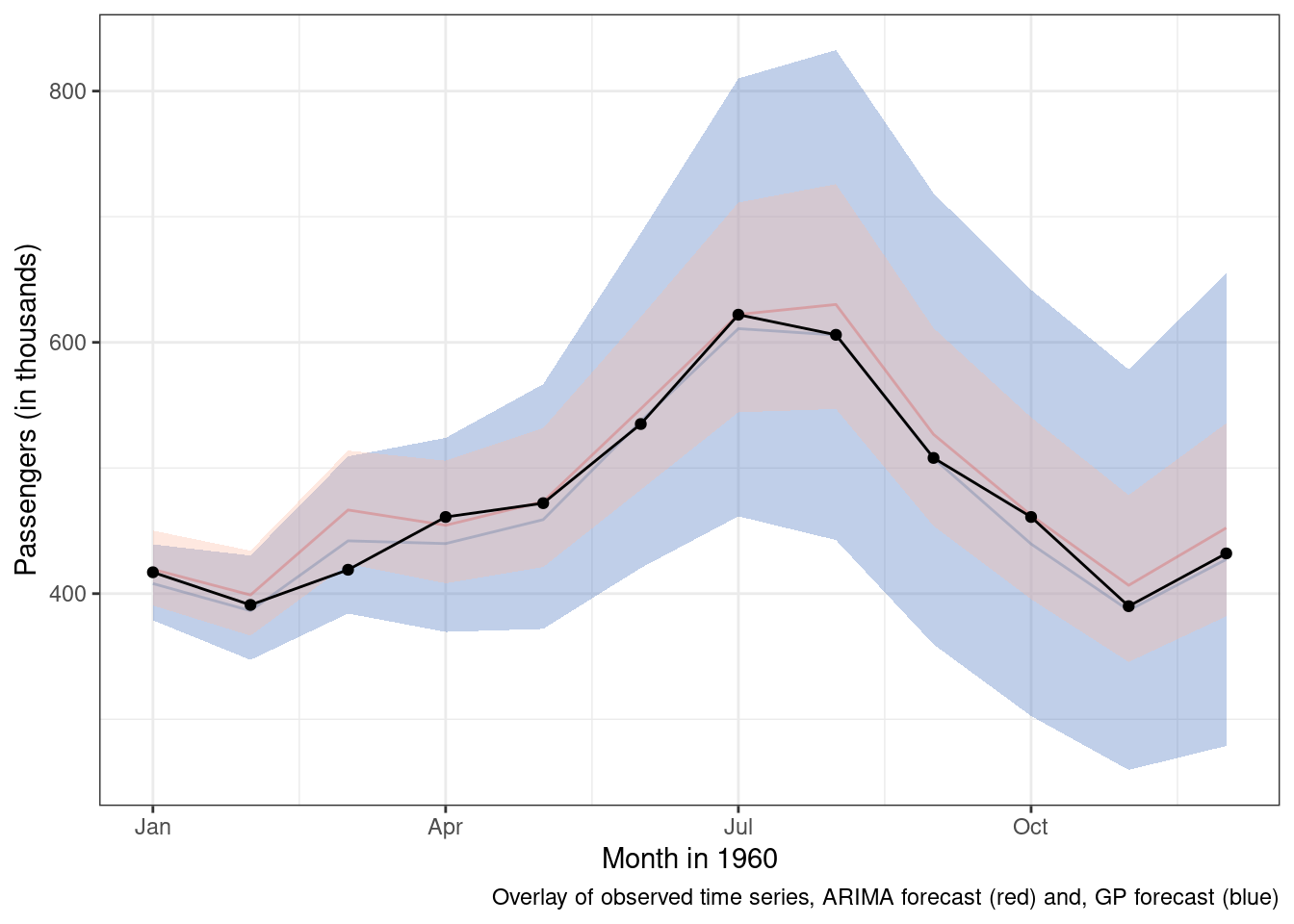
)And here are the results overlayed on top of the m4 predictions and observed data.
Some key differences 1. The ARIMA takes a lot less time to execute. Gaussian process models are unfortunately \(O(N^3)\), which means that as the number of data points increases the computational burden increases at an exponential rate. 1. The ARIMA model’s mean forecast is similar, but slightly worse than the Gaussian process model. 1. The ARIMA model is more certain about its predictions and while uncertainty does increase over time, the increase is not as pronounced.
If we are going to mainly use the mean predictions for forecasting, then the Gaussian process model appears to outperform our ARIMA results. If we care about uncertainty around the mean predictions, the two models have slightly different ideas about the range of plausible values in the future. If I were continuing on this modeling journey, that is where I would pivot to next.
Summary
This post has reviewed how to build a Gaussian process model to forecast an outcome of interest (monthly passengers) using only historical data measured at equal intervals over time. Hopefully, you are convinced that, with some oversight and judicious modeling, Gaussian processes can be combined to make effective time-series forecasts. The modeling technique is incredibly flexible, and, if there is a pattern that is discernible in the time-series, there is a Gaussian process and kernel function that can be used to represent it.
There are two cautionary notes that come with this flexibility. The first is that, in operating mainly on co-variance matrices, there are some computationally expensive steps that can be prohibitive in large data sets. The second is that, with an infinite number of Gaussian processes that could be used to model the data, it takes some work to ensure that only those that are relevant for the forecasting problem are used. In using these models, we need to guard against the risk of fitting a Gaussian process to random noise.